1. Introduction

1.1. Origin of the problem

Our residential community recently underwent a change in the homeowners' committee. As my father actively participated in the committee’s re-election and frequently engaged in discussions about property management, he was unanimously elected as the chairman. To select a suitable property management company for our community, he began conducting in-depth research into various property management companies in surrounding neighborhoods, their services, pricing standards, and fee structures. Watching my father devote himself tirelessly to these tasks, I realized that I had never seriously considered these issues before. This experience sparked my curiosity and inspired me to explore the topic further. I discussed with my father the possibility of conducting an in-depth study on property management-related issues, aiming to derive a scientific basis and formula for calculating property management fees. Encouraged and supported by my father, and after multiple discussions with both him and my mathematics teacher at school, I decided on the research topic: a mathematical model study on the optimal allocation of property management personnel, pricing strategy, and price adjustment mechanism.

1.2. Research approach

The early stage of this project involved field research in two residential communities in Shanghai, focusing on personnel allocation and economic management data. In the middle stage, three mathematical models were developed: an optimal allocation model for property management personnel, a pricing model for property management fees, and a customer satisfaction model for property management. In the final stage, the study focused on constructing a mechanism for the adjustment of property management fees.

Personnel allocation in property management should be based on both the specific characteristics of the project and the service requirements of the client (either the developer or the homeowners' committee). In other words, staffing should align with the content, frequency, and standards of the property management work. Following this, a cost structure analysis of property management is carried out to build a pricing model based on the optimized personnel allocation and cost analysis. Next, the factors influencing customer satisfaction with property management are analyzed to construct a satisfaction model, which is then linked to the pricing model. Finally, the study explores the mechanisms for adjusting service prices, aiming to systematically identify the factors influencing homeowners’ responses to such changes. Based on these insights, the adjustment model and its process are optimized to effectively guide the property service market toward a dynamic and responsive pricing system.

1.3. Research objectives

This research has four primary objectives:

• To determine personnel allocation based on the content, frequency, and standards of property management tasks, and to construct a mathematical model for optimal allocation. This model is then validated using real data from two residential communities in Shanghai.

• To analyze the cost structure of property management and construct a mathematical pricing model based on the optimal personnel allocation and cost analysis, with consideration of homeowner satisfaction.

• To identify the factors influencing homeowner satisfaction, use MATLAB to compute the weights of these factors, and build a satisfaction model that is linked to the pricing model.

• To explore the adjustment of property management fees by constructing a mathematical model and mechanism that balances the interests of both the property management company and homeowners in a rational and scientific manner.

1.4. Innovations

The innovative aspects of this study are summarized as follows:

• It provides a comprehensive and systematic analysis of property management, covering optimal personnel allocation, pricing strategies, satisfaction modeling, and price adjustment mechanisms.

• It proposes a personnel allocation model based on the specific content, frequency, and standards of property management tasks, and validates the model using real-world case studies.

• It conducts multi-sample analysis of property management costs and multi-factor analysis of customer satisfaction, constructing both a pricing model and a satisfaction model. Multiple methods for determining factor weights in the satisfaction model are also explored.

• For the first time, this study links the pricing model with the satisfaction model to establish a full-cost pricing approach based on homeowner satisfaction, resulting in a more scientific pricing method.

• It builds a price adjustment mechanism model that incorporates tax policies and the reasonable profit margins of property management companies.

2. Optimal allocation algorithm for property management personnel

The optimal allocation algorithm for property management personnel refers to the Equivalent Working Hour Method. Taking the allocation of security personnel as an example, it has been common practice in the industry to staff security based on area or number of households—such as assigning one security guard for every 5,000 square meters or 50 households. However, [1] argues that staffing should be based on both the characteristics of the project and the service requirements of the client (developer or homeowners’ committee) to be truly reasonable. More specifically, the allocation should consider the content, frequency, and standards of security work for the project.

Security services in property management generally include three main categories: gate duty, patrol of public areas, and monitoring room duty. Each of these categories may further be divided into subcategories depending on the actual situation of the project. For example, in a residential community, gate duty might include a main entrance post and a secondary entrance post.

For the same type of property, the frequency and standard of services (such as gate duty at the main entrance) are typically consistent. Furthermore, the service standards directly influence the required service frequency and time. For instance, if the standard specifies “24-hour duty and registration system at all entrance posts,” then higher frequency and intensity of service are required, which means more working hours. Conversely, if the standard allows the main entrance to be manned 24 hours and the secondary entrance only 16 hours, with a simple registration process, then fewer working hours are needed.

Therefore, when setting the frequency (i.e., daily work hours such as 24, 12, or 8 hours) and standards (i.e., work hours per shift, such as 8 hours) for security tasks, it is essential to fully consider the client’s basic service requirements.

Most of the daily tasks of property management security personnel—excluding emergencies such as thefts, fires, etc.—are regular and manageable in terms of frequency and workload.

2.1. Equivalent working hour method for optimal personnel allocation

Based on the principles above, the Equivalent Working Hour Method for optimal personnel allocation can be summarized in Table 1:

Table 1. Formulas for the equivalent working hour method

Note: According to company policy, a security guard works 26 days per month and 8 hours per day. To accommodate emergency responses and unscheduled inspections, a security team leader and patrol leader may also be assigned in addition to the regular guards. These leaders help ensure emergency response readiness, routine inspection coordination, and continuous service quality.

2.2. Case study of optimal personnel allocation and actual implementation

2.2.1. Case 1: a residential community in Jing’an District

This community consists of two 30-story residential buildings, covering a land area of 6,514 square meters with a total built area of approximately 40,000 square meters and 254 households. The personnel allocation calculation is shown in Table 2:

Table 2. Case calculation using the equivalent working hour method

Notes:

① The gate duty covers only the main entrance with two guards on duty 24/7 in 12-hour shifts.

② Patrols are conducted every 2 hours by two personnel, with each patrol lasting 0.6 hours.

③ The monitoring room is manned by two personnel 24/7.

④ 12-hour shifts with a 6-days-on, 1-day-off rotation were adopted.

Survey Results for Case 1:

• 12-hour shifts with a 6-days-on, 1-day-off rotation were adopted.

• Staffing considered labor contract terms to ensure stability.

• The monitoring room was merged with the main entrance post. After this adjustment, a total of 3 guards were on duty 24/7, covering gate duty, patrol, and monitoring. Therefore, monthly staffing = 3 × 24 × 31 / (31 × 6/7 × 12) ≈ 7 full-time security personnel.

• Occasionally, 1–2 temporary workers were hired during holidays or in times of increased workload (e.g., during the pandemic). Without additional workers, some staff had to work overtime.

2.2.2. Case 2: a second residential community in Jing’an District

Completed in 2005, this community has 10 buildings, each 38 stories tall, with a total built area of approximately 160,000 square meters (see Table 3).

Table 3. Case calculation using the equivalent working hour method

Notes:

① The gate duty covers only the main entrance with two guards on duty 24/7 in 12-hour shifts.

② Patrols are conducted every 2 hours by two personnel, with each patrol lasting 0.6 hours.

③ The monitoring room is manned by two personnel 24/7.

④ 12-hour shifts with a 6-days-on, 1-day-off rotation were adopted.

Survey Results for Case 2:

• Shift system: 12-hour shifts with one day off per week.

• Due to the larger area, two additional floating guards were added, bringing the total to 19 + 2 = 21 full-time security staff.

2.3. Conclusion

• The Equivalent Working Hour Method for personnel allocation is scientifically sound and allows for real-time adjustments, making it more practical than simply allocating based on area.

• Staffing should fully consider the actual conditions of each community, the affordability of property fees, and the local labor market when determining optimal personnel allocation.

• Unforeseeable events such as pandemics and staff absences require monthly, quarterly, and annual planning and adjustments.

• In general, there is no direct proportional relationship between community size and security labor costs. Larger communities often have lower labor costs per unit area, explaining why large communities in Shanghai can maintain good service quality with relatively low property fees.

3. Full-cost pricing model

After completing the study on the optimal allocation algorithm for property management personnel, we need to further construct a pricing model for property management fees based on this algorithm.

3.1. Comparison of pricing models

Pricing methods are specific approaches adopted by enterprises to achieve their pricing objectives. According to reference [3], a pricing method should include two aspects: price formation and price adjustment. These two jointly influence the development of a pricing model, which ultimately leads to the final price.

Among the commonly used pricing models, the authors have chosen the full-cost pricing method based on their research and an analysis of the advantages and disadvantages of various models. A comparison of conventional pricing models is shown in Table 4.

Table 4. Comparison of common pricing models

3.2. Revenues and expenditures of property management companies

As service providers, property management companies offer paid service products. Homeowners, as service recipients, are obliged to pay service fees based on the level of benefit received. Homeowners pay a fixed property management fee periodically, and property management companies determine the fee amount based on service costs, statutory taxes, and target profit margins. Only when revenues and expenditures are balanced can the company maintain normal operations.

Property management revenues are relatively straightforward. They consist of service fees and public benefit income, as shown in Table 5.

Table 5. Revenue categories of property management companies

In general, these revenue streams are relatively stable. Property service fees usually remain unchanged for several years, and parking fees are typically fixed. When fee levels are not adjusted, total revenue depends directly on collection rates.

In terms of expenditures (i.e., costs), personnel expenses constitute the largest portion, typically accounting for 60% to 70%. The average annual wage of personnel has been increasing at a rate of 5% to 10%, while the CPI has been growing at 3% to 5% annually. Utility costs such as water, electricity, and gas are also adjusted each year. As property management costs continue to rise rigidly and rapidly, while service fees remain unchanged, scientific pricing methods are increasingly essential.

Based on analysis of bidding documents from multiple property management companies in two surveyed communities, the major cost components are summarized as follows in Table 6.

Table 6. Cost categories of property management companies

3.3. Full-cost pricing method

Scientific pricing typically involves a combination of cost, supply and demand, and competition factors. According to literature [3], commonly used pricing methods include elastic pricing, shadow pricing, supply-demand pricing, income capitalization, etc. Among these, and based on the advantages and disadvantages of each approach, as well as field survey results and the specifics of the property management industry, the authors have chosen the full-cost pricing method. Based on research across several residential communities and property management companies in Shanghai, the authors summarized and derived the following formula for full-cost pricing (Table 7):

Table 7. Full-cost pricing model based on optimal staffing algorithm

Where:

P: Total cost of property management services for the community (unit: CNY)

U: Unit price of property management services (unit: CNY/square meter)

A: Total area subject to property management fees in the community (unit: m²)

P1: Total labor cost for the community (CNY)

P2: Total office expenses for the community (CNY)

P3: Total maintenance costs for equipment and facilities (CNY)

P4: Total public utility expenses (CNY)

P5: Total order maintenance costs (CNY)

P6: Total landscaping maintenance costs (CNY)

P7: Total environmental cleaning costs (CNY)

P8: Total insurance costs (CNY)

P9: Total miscellaneous expenses (CNY)

P10: Total management fee (CNY)

P11: Total statutory tax expense (CNY)

3.4. Full-cost pricing method based on resident satisfaction

Resident satisfaction with property services is determined by three dimensions: expectations of service, perceived quality of service, and perceived value of service. In simple terms, residents assess whether the property services they receive are equivalent to the fees they pay. Thus, service fee items become the "checklist" by which residents evaluate service quality.

The next section will discuss the satisfaction evaluation model in detail. This model categorizes resident satisfaction into five levels, as shown in Table 8.

Table 8. Satisfaction evaluation scale

In conjunction with the next section, we recommend that property pricing strategies should aim to ensure satisfaction scores above 80 points.

4. Property management satisfaction model

Residents’ satisfaction with property management directly affects their sense of gain and well-being. However, how to objectively express and evaluate the subjective factor of satisfaction has been rarely discussed in existing literature. According to Reference [4], the 1–9 scale method is a scientific approach most suitable for objectively expressing and evaluating various subjective factors. This paper attempts to apply methods based on junior-level algebra (systems of equations) or higher-level applied mathematics (linear algebra) to solve the problem.

4.1. Construction of a satisfaction evaluation index system based on the AHP method

Resident satisfaction with property management services is determined by three dimensions: service expectations, perceived service quality, and perceived service value. To explore resident satisfaction, it is essential to examine satisfaction with the major aspects of property management, and to analyze the weights of the influencing factors behind these aspects. Only then can the key factors influencing satisfaction be identified. The Analytic Hierarchy Process (AHP) is well-suited to solving this problem. The AHP model decomposes a complex problem into multiple components, which are then structured into different layers and groups according to their attributes. Elements within the same layer are independent of each other. Elements in the lower level represent different aspects of the higher-level elements and determine them. Therefore, the "goal layer"—residential property management satisfaction—is decomposed into several aspects (criteria layer), and the influencing factors of each aspect form the sub-criteria layer. By constructing the index system and conducting empirical research, this approach enables the identification of key issues and causes affecting residential property management satisfaction, thus informing targeted improvement suggestions.

1. Based on expert consultation and field surveys, Reference [4] identifies four aspects that residents care most about: management of shared areas and facilities, community public order, environmental services, and property fee collection. These four aspects are taken as the first-level (criteria) indicators in this study.

2. Reference [4] selects secondary indicators through expert consultation. The experts are chosen according to three principles: First, they must have extensive experience and authority in the field of property management. Second, both industry regulators and seasoned practitioners should be included, ideally along with academic experts. Third, the number of experts should be limited to 10–20. The composition of the expert panel is shown in Table 9:

Table 9. Composition of expert panel

3. Based on the results of expert meetings, an evaluation index system was constructed using the AHP method to support decision-making and determine overall satisfaction. The goal layer (A) is "property management satisfaction"; the criteria layer (B) includes satisfaction with shared area and facility management (B1), community public order (B2), environmental services (B3), and property fee collection (B4). Each criterion in B1–B4 corresponds to sub-criteria in layer C. The hierarchy is shown in Figure 1:

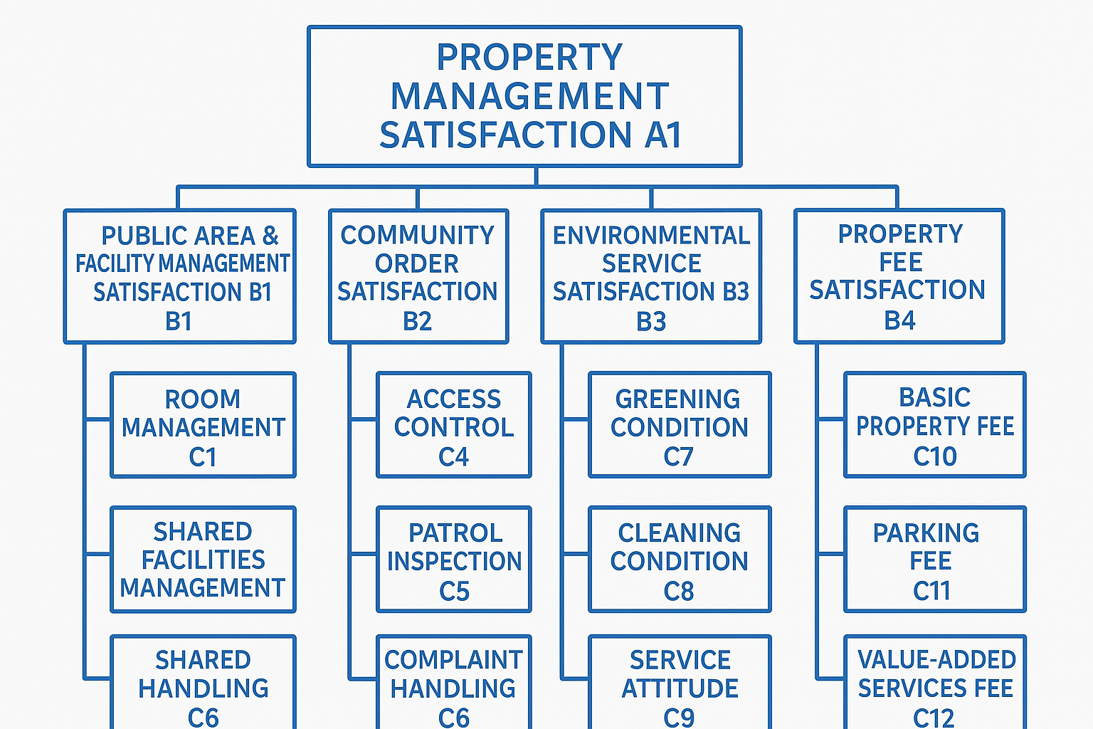
Figure 1. AHP hierarchical structure of the property management satisfaction evaluation system

4.2. Construction of judgment matrices

Elements at the same level and within the same group are compared pairwise to determine their relative importance. These comparisons are then quantified to construct judgment matrices. In this study, the 1–9 scale method is used to form the matrices based on expert pairwise comparisons.

This study uses five qualitative levels—"equally important," "slightly more important," "moderately more important," "significantly more important," and "extremely more important"—to differentiate the strength of comparisons between factors. These correspond to the standard 1–9 AHP scale, as shown in Table 10:

Table 10. 1–9 Ratio scale

Table 11. Judgment matrix between A and B layers

Table 12. Judgment matrix between B1 and its sub-criteria

Table 13. Judgment matrix between B2 and its sub-criteria

Table 14. Judgment matrix between B3 and its sub-criteria

Table 15. Judgment matrix between B4 and its sub-criteria

4.3. Calculation of weights and consistency check

4.3.1. Weight calculation using systems of equations

Assuming complete consistency in the five judgment matrices mentioned above (see Table 11-15), systems of equations were established and solved accordingly, as shown in Table 16:

Table 16. Weight calculation via systems of equations

Judgment matrices are derived through pairwise comparisons of elements at each hierarchical level based on their relative importance. However, due to the complexity of the real world and the diversity of human cognition, along with the absence of fixed references in pairwise comparisons among n elements, subjective inconsistencies may arise. Since systems of equations cannot verify consistency, it is more scientific and rational to employ matrix calculations and consistency tests based on advanced engineering mathematics.

4.3.2. Matrix-based weight calculation and consistency verification

Based on the constructed judgment matrices, the "root method" was used for weight calculation, wherein weights (i.e., eigenvectors) were derived using geometric mean and normalization. As matrix construction and consistency checks involve advanced mathematical concepts beyond the author's current academic level, the computations—under expert guidance—were performed using MATLAB software to obtain eigenvectors, the largest eigenvalue (λmax), and consistency ratios.

The constructed judgment matrix A must satisfy not only reciprocal properties but also consistency, i.e.,

\( {a_{ij}}{a_{jk}}={a_{ik}},∀i,j,k=1,2,...,n \) (1)

Typically, consistency is assessed by calculating the Consistency Ratio (CR):

\( CR=CI/RI \) (2)

When CR < 0.1, the consistency is deemed acceptable. If CR ≥ 0.1, the judgment matrix must be reconstructed. The Consistency Index (CI) is calculated from the matrix as:

\( CI=({λ_{max-n}})/(n-1) \) (3)

The Random Index (RI) values for matrices of different sizes are shown in Table 17:

Table 17. RI values for different matrix orders

Using MATLAB (see Figure 2):

The data is input in MATLAB as \( a=[….] \) , with elements separated by spaces and rows separated by semicolons. Then the command \( [yd]=eig(a) \) is used, where \( d= Diagonal Matrix \) . The first value on the diagonal corresponds to the largest eigenvalue.

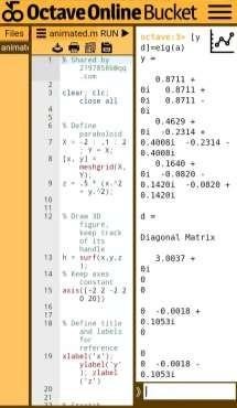
Figure 2. MATLAB interface for weight (eigenvalue) calculation

The weights and consistency test results for each hierarchical level calculated via MATLAB are shown in Tables 18 to 22:

Table 18. A-B layer weights and consistency test

\( {λ_{max}}=4.00 \) \( CR= CI/RI=0/0.9=0 \lt 0.1 \) , Acceptable

Table 19. B1-C layer weights and consistency test

\( {λ_{max}}=3.0097 \) \( CR= CI/RI=0.0048/0.58=0.0082 \lt 0.1 \) , Acceptable

Table 20. B2-C layer weights and consistency test

\( {λ_{max}}=3.0037 \) \( CR= CI/RI=0.0001/0.58=0.0017 \lt 0.1 \) , Acceptable

Table 21. B3-C layer weights and consistency test

\( {λ_{max}}=3.0193 \) \( CR= CI/RI=0.00965/0.58=0.0166 \lt 0.1 \) , Acceptable

Table 22. B4-C layer weights and consistency test

\( {λ_{max}}=3.0027 \) \( CR= CI/RI=0.00136/0.58=0.00234 \lt 0.1 \) , Acceptable

The combined weights (W) were calculated by multiplying the weights of the C-layer indicators by the corresponding B-layer weights. After consistency verification, the final weights across the A-C levels are shown in Table 23:

Table 23. A-C layer combined weights and consistency test

4.4. Design and empirical analysis of the satisfaction survey questionnaire

This study classifies satisfaction evaluation into five levels. The corresponding scores and classification criteria are detailed in Table 24.

Based on the constructed satisfaction evaluation index system and assessment methodology, the author conducted an additional WeChat-based online satisfaction survey targeting homeowners of Residential Community Case II in Jing’an District, Shanghai—who had previously participated in offline investigations. The questionnaire design is provided in Appendix 1. The online survey was distributed via group messaging, resulting in the collection of 34 responses (see Figure 3), all of which were valid, yielding a 100% response rate. After processing the data from the 34 questionnaires, average values were calculated for each of the 12 indicators across 12 observation points. Based on these averages, the overall satisfaction level of homeowners with residential property management services in Shanghai was computed.

Figure 3. Age distribution of survey respondents

Table 24. Satisfaction indicator calculations

By substituting the obtained average values into the residential property satisfaction evaluation index system and performing a weighted calculation, the sample property management satisfaction score was determined to be 73.17.

The results indicate that residents’ satisfaction with property management services is 73, falling within the “satisfied” category. However, this score lies near the lower threshold of the satisfaction range and remains considerably distant from the “very satisfied” level. This suggests that there is still significant room for improvement and enhancement in the quality of property management services in Shanghai.

5. Pricing adjustment model for property management

Research on the influencing factors of property management price adjustments mainly covers three aspects: external environmental factors, internal environmental factors, and other influencing factors. External factors primarily include economic conditions, the political environment, and market supply and demand. Internal factors are mainly related to project operation cost control and performance. Additionally, from the consumer perspective, demographic characteristics and perception of the service can also influence price adjustments.

5.1. Comparison of price adjustment models based on cost changes

Price adjustment models based on cost changes mainly consider variations in operational costs during the project period (see Table 25).

Table 25. Comparison of cost-based price adjustment models

Where:

Pt—Adjusted property management price during period

Pt-1—Property price in the previous period

CPI—Consumer Price Index

w—Raw material costs

s—Labor costs

p—Management fees

t—Statutory taxes

① ℎ1､ℎ2—Weights assigned to each cost factor(ℎ1+ ℎ2= 1)

② In Equation (2), ℎ₁, ℎ₂, and ℎ₃ represent the weights of material costs, labor costs, and the Consumer Price Index (CPI) in influencing changes in operating costs, respectively.(It is assumed that all other costs, apart from raw materials and wages, are reflected by the CPI.) The weights satisfy the condition:,ℎ 1 + ℎ2+ ℎ3=1｡

③ In Equation (3), ℎ₁, ℎ₂, ℎ₃, and ℎ₄ represent the weights of material costs, labor costs, management fees, and statutory taxes in influencing changes in operating costs, respectively. The specific values are as follows: ℎ1=0.23, ℎ2=0.65, ℎ3=0.06, ℎ4=0.06 which satisfy the condition:(ℎ1+ ℎ2+ ℎ3+ ℎ4= 1)

In the preceding sections discussing the full cost pricing method, the costs incurred by property management companies were categorized into 11 subcategories. These subcategories are further grouped into four major categories for modeling purposes: Labor costs; Raw material costs (including office expenses, equipment maintenance costs, public utility expenses, security maintenance costs, landscaping maintenance, environmental cleaning, insurance, and miscellaneous expenses); Management fees, and Statutory taxes. Accordingly, Formula 3 incorporates both management fees ppp and statutory taxes ttt, with assigned weights of ℎ₃=0.06 and ℎ₄=0.06, respectively. Additionally, since the CPI (Consumer Price Index) impact is inherently reflected in the growth rates of labor and raw material costs during the price adjustment period, the author argues that there is no need to separately factor in the CPI. Given that labor costs typically account for 60–70% of total costs, the weight for labor cost ℎ₂is set at the midpoint value of 0.65. Management fees are assigned a fixed weight of 0.06, and statutory taxes—being subject to policy—are also given a current fixed weight of 0.06. Consequently, the raw material cost weight ℎ₁is calculated as 0.23, resulting in the finalized version of Formula 3 as presented earlier.

5.2. Price adjustment calculation: a case study of a residential community in Jing’an district

The community comprises: Ground floor area: 1,237.72 m² (unit price: ¥6/m²/month); Upper floors area: 35,697.21 m² (unit price: ¥6.75/m²/month); Underground fixed parking spaces: 100 units (¥100/month); Surface parking spaces: 25 units (¥600/month, with 20% of the fee attributed to the property management company); The annual income is ¥3,136,589.85.

2023 expenditures are as follows: Raw material costs (w): ¥680,953.44; Labor costs (s): ¥2,060,379.72; Management fees (p): ¥151,944.73; Statutory taxes (t): ¥144,663.89; Total expenditure: ¥3,037,941.78

2024 forecast: Raw material costs (www): ¥701,382.04; Labor costs (sss): ¥2,142,794.91; Management fees (ppp): ¥151,944.73; Statutory taxes (ttt): ¥144,663.89; Projected total expenditure: ¥3,140,785.57.

Substituting these values into the formula below:

\( {P_{t}}={P_{t-1}}×({h_{1}}\frac{{w_{t}}}{{w_{t-1}}}+{h_{2}}\frac{{s_{t}}}{{s_{t-1}}}+{h_{3}}\frac{{P_{t}}}{{P_{t-1}}}+{h_{4}}\frac{{t_{t}}}{{t_{t-1}}}) \) (4)

\( {P_{t}}=3037941.78×(0.23\frac{701382.04 }{680953.44}+0.65\frac{2142794.91}{2060379.72}+0.06\frac{151944.73}{151944.73}+0.06\frac{144663.89}{144663.89}) \) (5)

This represents an approximate 3% increase over the 2023 level, which is below the expected profit margin. Compared to the actual projected 2024 expenditure, the deviation is less than 0.1%, indicating the high accuracy and practical applicability of the model.

6. Conclusion

6.1. Research achievements

This thesis has accomplished the following key objectives:

• Based on the content, frequency, and standards of property management tasks, a mathematical model for the optimal allocation of property management personnel was constructed. This model was empirically applied to two residential communities in Shanghai.

• The cost composition of property management was analyzed in depth. By integrating the optimal personnel allocation model with cost structure analysis, a pricing model for property management fees based on resident satisfaction was developed.

• The factors influencing resident satisfaction with property management services were identified and quantified using MATLAB. A mathematical model of satisfaction was constructed, and this model was then integrated with the pricing model to ensure consistency and practicality.

• A study was conducted on property service price adjustment mechanisms, resulting in the development of a mathematical model and pricing adjustment framework for property management fees.

6.2. Areas for improvement

Despite the achievements of this research, several limitations remain. The current models may not fully account for all possible influencing factors, and their applicability and accuracy require further validation. To address these limitations, the following improvement strategies are proposed:

• Consult more diverse modeling literature to incorporate a wider range of influencing factors into the models.

• Conduct broader surveys and field studies in additional residential communities within Shanghai to test the generalizability and precision of the proposed models.

6.3. Future prospects

This thesis represents the first comprehensive study of the entire property management process from a mathematical modeling perspective, resulting in a systematic set of models with significant potential for real-world application. Two directions for future research are envisioned:

• Continue to explore MATLAB as a computational tool, and further enhance the comprehensiveness and applicability of algorithms and models, thereby improving system accuracy and generalizability.

• Promote the widespread application of the models and methodologies proposed in this thesis across the property management industry to support scientific and standardized pricing and service optimization.

6.4. Personal reflections

Participation in this research project has been a deeply enriching experience. Key takeaways include:

• This was my first exposure to advanced engineering mathematics, including matrix operations, and the application of MATLAB as a computational tool.

• I gained a deeper understanding and strong interest in various types of mathematical models, providing a more intuitive grasp of algorithmic thinking and modeling techniques.

• Under the guidance of my supervisor, I learned the importance of academic rigor and standardization in thesis writing, which helped me develop a methodical and pragmatic research attitude.

References

[1]. Mao, Z., & Yan, Y. (2007). Allocation techniques for security personnel in property management. Modern Property Management, 15, 50–51.
[2]. Fu, H. (2018). A case analysis of activity-based costing in XXH Property Management Company (Master’s thesis). Chinese Academy of Fiscal Sciences.
[3]. Ou, L. (2015). Exploring the pricing dilemma and pricing methods of property fees in Wuhan: A case study of Xiangxie Shuian Community in Wuchang (Master’s thesis). Huazhong University of Science and Technology.
[4]. Jiao, D. (2018). A study on residential property management satisfaction in Dalian (Master’s thesis). Dalian University of Technology.
[5]. Tao, K. (2020). A study on influencing factors and mechanisms of property service price adjustments (Master’s thesis). Beijing Forestry University.
[6]. Zhang, H., & Chen, X. (2019). AHP-TOPSIS-based optimal evaluation method for property management bidding. Journal of Hubei University (Natural Science Edition), 41(3), 264–269.
Cite this article
Gao,Z. (2025). A mathematical model study on the optimal allocation, pricing strategy, and price adjustment mechanism of property management personnel. Advances in Social Behavior Research,16(3),113-127.
Data availability
The datasets used and/or analyzed during the current study will be available from the authors upon reasonable request.
Disclaimer/Publisher's Note
The statements, opinions and data contained in all publications are solely those of the individual author(s) and contributor(s) and not of EWA Publishing and/or the editor(s). EWA Publishing and/or the editor(s) disclaim responsibility for any injury to people or property resulting from any ideas, methods, instructions or products referred to in the content.
About volume
Journal:Advances in Social Behavior Research
© 2024 by the author(s). Licensee EWA Publishing, Oxford, UK. This article is an open access article distributed under the terms and
conditions of the Creative Commons Attribution (CC BY) license. Authors who
publish this series agree to the following terms:
1. Authors retain copyright and grant the series right of first publication with the work simultaneously licensed under a Creative Commons
Attribution License that allows others to share the work with an acknowledgment of the work's authorship and initial publication in this
series.
2. Authors are able to enter into separate, additional contractual arrangements for the non-exclusive distribution of the series's published
version of the work (e.g., post it to an institutional repository or publish it in a book), with an acknowledgment of its initial
publication in this series.
3. Authors are permitted and encouraged to post their work online (e.g., in institutional repositories or on their website) prior to and
during the submission process, as it can lead to productive exchanges, as well as earlier and greater citation of published work (See
Open access policy for details).