1. Introduction

Balancing global economic growth with environmental sustainability has become the focus of international attention. The signing of the Paris Agreement and the convening of COP26 marked a new historical stage in global climate governance, prompting nations to commit to more ambitious emissions reduction targets [1]. As a key participant in global climate governance, China officially proposed the carbon peaking goal by 2030 and the carbon neutrality goal by 2060. These targets not only reflect China’s responsibility as a major power but also clearly set the direction for regional low-carbon transitions.

In the process of carbon reduction, urban agglomerations—core areas of regional economic development—have increasingly emphasized the importance of scientifically measuring and evaluating their carbon emission performance. With accelerating urbanization, urban agglomerations concentrate large populations, industries, and resources, amplifying their environmental impacts. Therefore, establishing a systematic evaluation method for carbon emission efficiency and improving the performance of urban agglomerations are crucial for promoting a nationwide green transformation [2, 3]. In China, both the “14th Five-Year Plan” and the third plenary session of the 20th CPC Central Committee have emphasized coordinated development among urban agglomerations, providing policy support for research on carbon emission performance.

However, significant disparities exist among urban agglomerations in terms of scale, developmental stages, risk resilience, and environmental resilience management, resulting in pronounced regional and phased differences in input-output performance [4]. Mature urban agglomerations, such as the Guangdong-Hong Kong-Macao Greater Bay Area and the Yangtze River Delta, have established advanced market-oriented emission reduction mechanisms due to their developed economic foundations, technological capabilities, and effective management systems. In contrast, emerging urban agglomerations face considerable challenges in improving carbon emission performance due to constraints related to their development stages and industrial structures. Given rapid changes in regional economic conditions and industrial layouts, traditional “one-size-fits-all” emission reduction strategies are insufficient for clearly identifying performance levels and evolutionary trends across diverse urban clusters, necessitating more precise evaluation methodologies.

2. Literature review

Research methodologies for evaluating carbon emission performance have evolved from simple single-indicator measures to multi-factor evaluations and, more recently, to non-parametric methods based on production frontier theory. Early research primarily relied on indicators such as carbon emissions per unit of GDP or carbon intensity to assess the economic impacts of emissions [5, 6]. For example, Sun analyzed performance based on the rate of change in carbon intensity, providing preliminary insights for dynamic evaluation [7]. However, such indicators fail to fully capture the complexity and dynamics of carbon emissions within economic systems.

To address these shortcomings, multi-factor evaluation methods gained prominence. Early studies widely adopted the Malmquist and Luenberger indices for dynamic productivity analysis. Initially proposed by Färe et al., the Malmquist index assesses productivity changes over time [8]. Zhang et al. further developed a multidimensional framework, including cumulative per capita carbon emissions and carbon intensity per GDP, thereby improving comparative analyses across regions. Although these approaches handle complexity better, they still rely heavily on weighting schemes and data quality, which limits their effectiveness in dynamic and unobservable-factor analyses.

Subsequently, non-parametric methods based on production frontier theory provided significant methodological advancements. Data Envelopment Analysis (DEA), introduced by Charnes et al. and Banker et al, became crucial for environmental performance evaluation due to its flexibility in simultaneously handling desirable and undesirable outputs without assuming production functions [9, 10]. Färe et al. introduced Directional Distance Functions (DDF) for evaluating pollutant emissions, although their radial assumption limited practical flexibility. The Non-Radial Directional Distance Function (NDDF), later developed by Färe & Grosskopf and Zhou et al., allows varying proportions between desirable and undesirable outputs, better reflecting real-world economic activities [11, 12]. Based on NDDF, Meng and Wu et al. analyzed regional carbon emission performance, validating the applicability of NDDF. Furthermore, spatial heterogeneity and temporal dynamics have become focal points in research, with studies by Liu et al., Che et al., and Xie et al. emphasizing spatial correlations, technological innovation, and policy interactions, advancing research on regional carbon reduction and dynamic evolution patterns.

Despite numerous studies addressing carbon emissions with significant advances in methods and spatial-temporal analyses, some gaps remain. Firstly, most research focuses on single-city or provincial scales, lacking systematic comparative analysis across larger spatial scales encompassing multiple urban agglomerations. Secondly, even research addressing urban agglomerations predominantly relies on macro-level discussions or case studies, neglecting rigorous quantitative evaluations across varying periods, scales, and regional conditions [13]. Third, although some studies integrate NDDF with the Malmquist index, systematic explorations of the overall volatility trends and drivers of urban agglomerations' carbon emission performance remain limited.

To bridge these gaps, this study employs NDDF to measure the carbon emission efficiency of 16 national-level urban agglomerations in China from 2006 to 2022, integrating a Global Malmquist-Luenberger (GML) index for dynamic decomposition. This paper contributes methodologically and theoretically by: (1) constructing an accurate carbon emission performance index using NDDF, overcoming limitations inherent in traditional radial efficiency measures; (2) applying the GML index to differentiate the impacts of efficiency changes and technological progress, and utilizing the Dagum Gini coefficient to identify inequality sources among urban agglomerations; and (3) providing empirical evidence on the spatial patterns and temporal evolution of carbon emission performance, thereby offering a scientific foundation for identifying replicable and generalizable paths towards regional carbon peak strategies.

3. Research methodology and data processing

3.1. Research methodology

3.1.1. DEA efficiency analysis

In order to more accurately measure the carbon emission performance of urban agglomerations and their dynamic evolution, this paper makes methodological improvements based on existing studies. First, following the productivity decomposition idea of Färe et al. (1996), the desired and undesired outputs are included in the technological production set in order to account for carbon emission control when evaluating economic performance [14]. Accordingly, the technology production set is defined as follows

\( T=\lbrace (L,K,E,GDP,{CO_{2}}):(L,K,E) can produce (GDP,{CO_{2}})\rbrace \ \ \ (1) \)

Equation (1) shows that inputs of labor ( \( L \) ), capital ( \( K \) ), and energy ( \( E \) ) lead to a desired output, Gross Domestic Product ( \( GDP \) ), and an undesired output, carbon dioxide ( \( {CO_{2}} \) ). Following the assumptions of Färe et al., desired outputs have strong disposability and undesired outputs have weak disposability and can be bounded under Constant Returns to Scale (CRS) or Variable Returns to Scale (VRS) [15]. If the technology production set is assumed to have constant returns to scale, it can be further expressed as follows:

\( T=\lbrace \begin{array}{c} (L,K,E,GDP,{CO_{2}}):\sum _{n=1}^{N}{λ_{n}}{K_{n}}≤K,\sum _{n=1}^{N}{λ_{n}}{K_{n}}≤K,\sum _{n=1}^{N}{λ_{n}}{E_{n}}≤E, \\ \sum _{n=1}^{N}{λ_{n}}{GDP_{n}}≥GDP,\sum _{n=1}^{N}{λ_{n}}{{CO_{2}}_{n}}={CO_{2}},{λ_{n}}≥0,n=1,2,…N \end{array} \rbrace \ \ \ （2） \)

Theoretically, compared with traditional parametric estimation methods (e.g., Stochastic Frontier Analysis SFA), nonparametric DEA has more flexibility and is particularly suitable for measuring efficiency that includes both desired and undesired outputs [16, 17].

In the specific measurement, the Directional Distance Function (DDF) is the key. Traditional radial models (e.g., CCR, BCC) usually assume that inputs or outputs change in the same proportion, and it is difficult to disaggregate the different adjustment margins of desired and undesired outputs [18]. After Chung et al. proposed the directional distance function, although it has expanded the idea of environmental performance measurement, it still belongs to the radial hypothesis. To overcome this shortcoming, NDDF allows desired output and undesired output to be adjusted in different proportions, which is closer to the diversified change characteristics of economic growth and pollution emission in reality. Therefore, this paper adopts NDDF to measure the carbon emission performance of urban agglomerations, which can be mathematically regarded as finding the optimal technological frontier and calculating the inefficiency distance by reducing \( {CO_{2}} \) emissions and increasing \( GDP \) by different proportions under the premise of given inputs.

3.1.2. NDDF measurement models

In this paper, we refer to both Zhou et al. (2012) and Shao et al. studies [12, 19] to define the following model with the expression:

\( \vec{D}(x,y,b;g)=sup{\lbrace {w^{T}}β:((x,y,b)+g\cdot diag(β))∈{A^{T}}\rbrace }\ \ \ (3) \)

In equation (3), the input vector denoted by \( x=(L,K,E) \) produces the desired output \( y=GDP \) and the undesired output \( b={CO_{2}} \) ; the set of all possible production technologies is denoted by \( {A^{T}} \) , which represents the transposition of the set of technological possibilities. where \( w={({w_{L}},{w_{K}},{w_{E}},{w_{GDP}},{w_{{CO_{2}}}})^{T}} \) is a vector of normalized weights associated with the number of inputs and outputs; Since we want the expected direction of efficiency improvement to be an increase in desired outputs, a decrease in inputs, and a decrease in non-desired outputs, in order to characterize the level of efficiency of the production units, the NDDF model is set to Direction vector \( g=(-{g^{x}},{g^{y}},-{g^{b}}) \) , denotes the direction of decreasing inputs, increasing desired outputs, and decreasing non-desired outputs, respectively; \( β={({β_{L}},{β_{K}},{β_{E}},{β_{GDP}},{β_{{CO_{2}}}})^{T}}≥0 \) denotes the scaling factor vector, and \( diag(β) \) denotes the diagonalization of the \( β \) vector.

Based on the basic assumptions of technology production set in Eq. (2), the DEA method is used in this study to solve the NDDF. The model can be obtained by solving the following linear programming problem, whose objective function and constraints are denoted as:

\( \vec{D}(x,y,b;g)=max({w_{L}}{β_{L}}+{w_{K}}{β_{K}}+{w_{E}}{β_{E}}+{w_{GDP}}{β_{GDP}}+{w_{{CO_{2}}}}{β_{{CO_{2}}}})\ \ \ (4) \)

\( s.t.\begin{cases} \begin{array}{c} \sum _{n=1}^{N} {λ_{n}}{L_{n}}≤L-{β_{L}}{g_{L}} \\ \sum _{n=1}^{N} {λ_{n}}{K_{n}}≤K-{β_{K}}{g_{K}} \\ \sum _{n=1}^{N} {λ_{n}}{E_{n}}≤E-{β_{E}}{g_{E}} \\ \sum _{n=1}^{N} {λ_{n}}GD{P_{n}}≥y+{β_{GDP}}{g_{GDP}} \\ \sum _{n=1}^{N} {λ_{n}}CO{2_{n}}=b-{β_{C{O_{2}}}}{g_{C{O_{2}}}} \\ {λ_{n}}≥0,n=1,2,…,N \\ {β_{L}},{β_{K}},{β_{E}},{β_{GDP}},{β_{C{O_{2}}}}≥0 \end{array} \end{cases}\ \ \ (5) \)

Equation (5) comprehensively considers key factors such as input slack, desirable output slack, undesirable output slack, and the weak disposability of undesirable outputs. Based on the given objectives, the direction vector \( g \) can be set in different ways. When \( \vec{D}(x,y,b;g)=0 \) , it indicates that the Decision-Making Unit (DMU) is on the optimal production frontier, meaning its input-output efficiency has reached the optimal level. The solution of this function primarily reflects the distance between the DMU and the frontier, which can thus be interpreted as an economic inefficiency index incorporating carbon dioxide emissions.

This study references the methods of Zhou et al., Zhang et al., and Shao et al. to set the direction vector as \( g=(-K,-L,-E,GDP,{-CO_{2}}) \) and adopts a balanced weight allocation strategy. Each input factor, desirable output, and undesirable output is assigned a weight of 1/3, further distributed evenly among the types of factors. The final weight vector is determined as (1/9,1/9,1/9,1/3,1/3) to ensure fair and reasonable evaluation of each factor's contribution within the model ^{[12, 20]}.

Using Equations (4) and (5), this study calculates inefficiency based on both the unified technology frontier constructed over the entire study period and the annual technology frontiers. According to the definitions of the reference set and data structure, two types of Non-Radial Directional Distance Functions (NDDF) are constructed: global \( \vec{{D^{G}}}(x,y,b) \) and current-period \( \vec{{D^{t}}}(x,y,b) \) .Constructing an independent production frontier for each year and calculating the inefficiency value \( \vec{{D^{t}}}(x,y,b) \) provides the relative efficiency level of urban agglomerations during that period, reflecting competition among agglomerations under given technological conditions. Alternatively, using pooled data from the entire study period to construct a unified frontier and calculate inefficiency values \( \vec{{D^{G}}}(x,y,b) \) yields a measure of relative efficiency under the long-term overall technological context, identifying gaps relative to the optimal technology. Furthermore, four distance function values corresponding to global and current-period measures for periods \( t \) and \( t+1 \) can be calculated separately.

Through NDDF, this study quantifies the extent to which each Decision-Making Unit (DMU) deviates from the optimal frontier in terms of inputs and outputs. These inefficiency measures are typically expressed as reductions or increases in inputs and outputs. From an economic perspective, the results of Equations (4) and (5) only reveal the potential for efficiency improvement when considering undesirable outputs such as CO₂. These calculated values, however, cannot directly measure the specific effectiveness of carbon emission control.

Current-period efficiency reflects short-term, contemporaneous relative performance, while global efficiency reflects long-term, overall efficiency positioning. Combining the two helps distinguish performance improvements driven by management efforts to approach the frontier (catch-up effect) from advancements in technology itself (frontier shift). Based on the ratio method of target carbon emissions to actual carbon emissions proposed by Zhou et al. and incorporating the intrinsic relationship of input-output slack variables in the production possibility frontier, the ratio of target carbon emissions to actual emissions is extended into a comprehensive indicator that accounts for GDP growth [12]. This Carbon Reduction Efficiency Index (CREI), calculated based on the annual production frontier, effectively measures the synergistic effect of achieving both economic growth and carbon emission reduction in urban agglomerations during a specific period. The formula is as follows:

\( {CREI^{t}}=\frac{({CO_{2}}-β_{C{O_{2}}}^{t}{CO_{2}})/(GDP+β_{GDP}^{t}GDP)}{{CO_{2}}/GDP}=\frac{1-β_{C{O_{2}}}^{t}}{1+β_{GDP}^{t}}\ \ \ (6) \)

Here the relaxation variables of the directional distance function of CO₂ emission and GDP, denoted by \( β_{C{O_{2}}}^{t} \) and \( β_{GDP}^{t} \) respectively, are derived from the solution of the NDDF model in the \( t \) period. The proposed Equation (6) overcomes the limitation of the traditional single-dimension evaluation by incorporating a weighted assessment of economic growth and emission reduction effects. The slack variable, being a dimensionless value, guarantees the comparability of measurement results across disparate decision-making units.

3.1.3. Malmquist processing and dynamic decomposition

The Malmquist-Luenberger (ML) index is commonly used to measure total factor productivity changes incorporating undesirable outputs [21]. However, traditional ML indices often suffer from infeasibility across periods or efficiency biases. To address these limitations, scholars have proposed the Global Malmquist-Luenberger (GML) index and the Biennial Malmquist-Luenberger (BML) index, introducing non-radial forms to mitigate angular and radial assumption constraints [20, 22-25]. Among these, the GML index, based on the global technology frontier, avoids non-circularity and partial biases inherent in the ML index, better capturing intertemporal technological changes and promoting dynamic and comprehensive performance measurement methods.

To evaluate the trends in Total Factor Carbon Emission Productivity (TFCEP) across periods, this study employs the Global NDDF to calculate the Global Malmquist-Luenberger (GML) index: \( {TFCEP\_GML_{t,t+1}}=\frac{1+\vec{{D^{G}}}({x^{t}},{y^{t}},{b^{t}})}{1+\vec{{D^{G}}}({x^{t+1}},{y^{t+1}},{b^{t+1}})}\ \ \ (7) \)

The advantage of the GML index lies in its ability to effectively address infeasibility issues in linear programming, providing a more robust measure of productivity growth (Zhou et al., 2012) [12]. In Equation (7), \( \vec{{D^{G}}}(x,y,b) \) is calculated based on the production frontier constructed using data from the entire study period (2006–2022), and it measures the inefficiency of each DMU relative to this global frontier. This reflects the long-term overall efficiency level and identifies DMUs that remain inefficient even under the global technological context. Here, \( {x^{t}},{y^{t}},{b^{t}} \) and \( {x^{t+1}},{y^{t+1}},{b^{t+1}} \) represent inputs, desirable outputs, and undesirable outputs for periods \( t \) and \( t+t \) respectively. If \( {TFCEP\_GML_{t,t+1}} \gt 1 \) , it indicates improved carbon emission performance from period t to \( t+1 \) ; if T \( {TFCEP\_GML_{t,t+1}} \lt 1 \) , performance has declined. By adopting the global technology frontier, the GML index avoids infeasible solutions inherent in the traditional ML index and better reflects long-term technological disparities.

The GML index can also be dynamically decomposed to identify spatiotemporal evolution patterns across multiple dimensions, such as efficiency change (EC) and technological change (TC):

\( {EC_{t,t+1}}=\frac{1+\vec{{D^{t}}}({x^{t}},{y^{t}},{b^{t}})}{1+\vec{{D^{t+1}}}({x^{t+1}},{y^{t+1}},{b^{t+1}})}\ \ \ (8) \)

\( {TC_{t,t+1}}=\frac{\frac{(1+\vec{{D^{G}}}({x^{t}},{y^{t}},{b^{t}}))}{(1+\vec{{D^{t}}}({x^{t}},{y^{t}},{b^{t}}))}}{\frac{(1+\vec{{D^{G}}}({x^{t+1}},{y^{t+1}},{b^{t+1}}))}{(1+\vec{{D^{t+1}}}({x^{t+1}},{y^{t+1}},{b^{t+1}}))}}\ \ \ (9) \)

while

\( {TFCEP\_GML_{t,t+1}}={EC_{t,t+1}}×{TC_{t,t+1}}\ \ \ (10) \)

In this decomposition, the EC indicator reflects the change in the efficiency of the decision unit on the technology frontier, while the TC indicator measures the movement of the technology frontier itself [26]. Among them, since each year possesses its own set of production possibilities and frontier, \( \vec{{D^{t}}}(x,y,b) \) is the result of the calculation of the production frontier constructed based on the separate data for each year, which measures the relative degree of inefficiency of the DMU under its own technological conditions in that year, which reflects the performance of the DMU in the current period in comparison with other decision-making units in the same period.

The setting for the study stipulates that the values of the GML index, EC, and TC are all greater than 0. Among them, when these values are greater than 1, it indicates that the carbon emission performance improves, and both technical efficiency and progress are positive. Conversely, if these values are less than 1, it signifies that the carbon emission performance declines, and both technical efficiency and progress regress. Furthermore, when EC is greater than 1, it signifies that efficiency enhancement predominates performance growth, while when TC is greater than 1, it indicates that technical progress predominates performance growth. The decomposition analysis employed in this study facilitates a more profound comprehension of the alterations in production efficiency and technology level of each decision-making unit across diverse periods. This analytical approach provides a robust foundation for the formulation of pertinent policies.

3.1.4. Spatial disparity analysis

To systematically analyze the spatial disparities in carbon emission performance across Chinese urban agglomerations, this study employs Dagum’s Gini coefficient decomposition and Kernel Density Estimation (KDE) to evaluate the CREI and GML indices.

Dagum’s Gini coefficient, an advanced measure of inequality proposed by Dagum, decomposes overall disparities into three components: within-group inequality, between-group inequality, and transvariation [27]. This method overcomes the limitations of traditional Gini coefficients by explicitly distinguishing between intra-group and inter-group disparities. In this study, Dagum’s Gini coefficient is applied annually to analyze inequality in performance metrics across the 16 urban agglomerations. This approach has been widely adopted in environmental economics and regional studies. For instance, the overall Gini coefficient and its decomposition for the current-period results are illustrated in Equations (11–14).

Kernel Density Estimation (KDE) is further used to visualize the dynamic evolution of carbon emission performance distributions. By estimating probability density functions non-parametrically, KDE captures shifts in central tendencies, dispersion, and multimodality of performance metrics over time. This combination of Dagum’s decomposition and KDE provides a comprehensive understanding of spatial heterogeneity and convergence patterns in carbon emission efficiency.

\( G=\frac{1}{2{n^{2}}\bar{{CREI^{t}}}}\sum _{i=1}^{n}\sum _{j=1}^{n}|CREI_{i}^{t}-CREI_{j}^{t}|\ \ \ (11) \)

\( G={G_{w}}+{G_{nb}}+{G_{t}}\ \ \ (12) \)

\( {G_{w}}=\sum _{j=1}^{k}\frac{{n_{j}}}{n}{G_{j}}\ \ \ (13) \)

\( {G_{nb}}=\sum _{j=2}^{k}\sum _{h=1}^{j-1}\frac{{n_{j}}{n_{h}}}{{n^{2}}}{d_{jh}}\ \ \ (14) \)

\( {d_{jh}}=\frac{1}{2\bar{{CREI^{t}}}}\int _{0}^{∞}\int _{0}^{∞}|CREI_{i}^{t}-CREI_{j}^{t}|{f_{j}}(CREI_{j}^{t}){f_{h}}(CREI_{h}^{t})dCREI_{j}^{t}dCREI_{h}^{t}\ \ \ (15) \)

The sample size n represents the number of urban agglomerations observed annually, corresponding to the annual data of 16 national-level urban agglomerations. \( \bar{{CREI^{t}}} \) denotes the mean CREI value for all urban agglomerations in a specific year, used to standardize the Gini coefficient calculation. \( CREI_{i}^{t} \) and \( CREI_{j}^{t} \) represent the carbon emission performance values of urban agglomerations \( i \) and \( j \) in a given year, respectively, measuring absolute disparities between them. Additionally, \( {n_{j}} \) indicates the number of urban agglomerations within the j-th classification group (e.g. categories such as “optimization-enhancing” type, “growth-enhancing” type, and “development-nurturing” type as defined in China's 14th Five-Year Plan 10)., while \( k \) denotes the total number of classification groups. These variables collectively form the foundation of Dagum’s Gini coefficient and its decomposition, ensuring accurate reflection of inequality in carbon emission performance and its sources. Equation (15) calculates the average absolute difference between the j-th and h-th classification groups.

3.2. Data collection and processing

3.2.1. Selection of research subjects

China's national-level urban agglomerations show significant heterogeneity in terms of geographic distribution, size hierarchy, and economic and geographic characteristics. According to the “14th Five-Year” New Urbanization Implementation Plan, there are currently 19 national-level urban agglomerations in China, whose spatial layout covers four major segments, namely the eastern coastal region (5 clusters), central region (3 clusters), western region (9 clusters), and northeastern region (2 clusters), and covers diversified geographical environments, economic structures and development stages, which can fully represent the typical characteristics of China's regional development. It can fully represent the typical characteristics of China's regional development. In addition, in order to more clearly reflect the development positioning and policy orientation of each urban agglomeration, this study divides the urban agglomerations into three categories based on the “Outline of the 14th Five-Year Plan for National Economic and Social Development of the People's Republic of China and the Visionary Goals for the Year 2035” (referred to as the “14th Five-Year Plan”): (1) “optimization-enhancing” type, including the Beijing-Tianjin-Hebei region, Yangtze River Delta region, Pearl River Delta region, Middle reaches of Yangtze River, and Chengdu-Chongqing region; (2) “growth-enhancing” type, comprising the Shandong Peninsula region, Zhongyuan region, Guanzhong Plain region, Beibu Gulf region, and Guangdong-Fujian-Zhejiang Coastal region; and (3) “development-nurturing” type, covering Harbin-Changchun region, Central and Southern Liaoning, Central Shanxi region, Central Guizhou region, Central Yunnan region, Huhhot-Baotou-Ordos-Yulin region, Lanzhou-Xining region, Ningxia region along the Yellow River, and North slope region of Tianshan Mountains. The classification of the 16 urban agglomerations is illustrated in Fig. 1, accompanied by the abbreviated pronouns for the urban agglomerations in the data tables below, which have been included to facilitate the presentation.

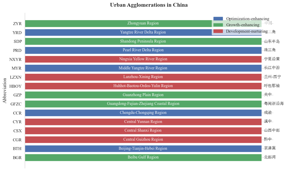
Figure 1. Abbreviation cross-reference for urban agglomerations in China

In terms of scale, urban agglomerations exhibit a clear gradient: the Beijing-Tianjin-Hebei and Yangtze River Delta regions, centered on Beijing and Shanghai, are ultra-large, while the Zhongyuan and Guanzhong Plain regions, anchored by Zhengzhou and Xi'an, are medium-sized. Additionally, each cluster develops distinct patterns based on resource endowments. For example, the Yangtze River Delta region excels in high-end manufacturing and modern services, while the Chengdu-Chongqing region focuses on equipment manufacturing and electronics. These differences further contribute to regional variations in carbon emission profiles [4].

In selecting the sample, this study adhered to the principle of data availability. Due to missing data or inconsistent starting years in statistical yearbooks, cities in the Harbin-Changchun region, Central and Southern Liaoning, and the North Slope region of the Tianshan Mountains—confirmed through correspondence with provincial statistical authorities—were excluded. As a result, 16 national urban agglomerations from 2006 to 2022 were selected. Their spatial distribution and economic-geographic characteristics still effectively reflect China's regional development patterns.

In defining the sample, this study cross-checked overlapping spatial boundaries. Six prefecture-level cities—Dezhou, Handan, Heze, Xingtai, Liaocheng, and Yuncheng—belong to two national urban agglomerations simultaneously. These cities were redundantly included in the statistics of their respective clusters. In the end, data were collected and compiled for 190 prefecture-level cities under the 16 urban agglomerations, whose spatial density and economic-geographic characteristics matched the typical requirements for national urban agglomeration development.

3.2.2. Selection of production indicators

The study adopts the Non-Radial Directional Distance Function (NDDF) to construct a closed-loop analytical framework of "input-output-emission." Capital, labor, and energy consumption are selected as input indicators, GDP as the desired output, and carbon emissions as the undesired output. This framework aligns with production function theory to comprehensively characterize urban production features and quantify carbon emission efficiency. The selection of capital, labor, and energy as inputs is based on two criteria: (1) their theoretical alignment with core production factors in economic theory, ensuring a comprehensive representation of urban production dynamics, and (2) their significant relevance to carbon emissions, as labor expansion correlates with energy intensity, while capital-intensive production and non-clean energy structures drive carbon emission intensity. Carbon emissions and GDP jointly form the output side of the production function, providing a theoretical foundation for quantifying carbon emission performance.

In terms of data collection, this study employs a multi-source integration approach. The primary data are sourced from the CSMAR and Wind economic databases, supplemented by provincial and municipal statistical yearbooks. To address missing values and variations in data collection standards, we employ cross-verification through statistical bulletins, historical growth-rate extrapolation, and literature-based calibrations (e.g., estimating missing values from year-on-year growth rates or using average values of comparable cities). The time span for the relevant input-output indicators extends from 2006 to 2022.

Regarding input indicators, annual employed population data at the prefecture level are used to measure labor, with interpolation methods applied to fill missing data and reconcile discrepancies in statistical standards. Capital stock is estimated via the perpetual inventory method, referencing the depreciation rate of 10.96% proposed by Shan, and deflated by constant base-period prices [28]. The formula is: \( {K_{i,t}}={I_{i,t}}+(1-δ){K_{i,t-1}} \) where \( {K_{i,t}} \) denotes the capital stock of city \( i \) in year \( t \) , \( {I_{i,t}} \) is the constant-price fixed-asset investment in year \( t \) , and \( δ \) is the depreciation rate, implying the current year's capital stock equals the sum of that year’s investment plus the net capital stock carried over from the previous year after depreciation. Energy consumption is estimated through a spatial downscaling model that uses the modified DMSP-OLS-like nighttime light dataset from Wu et al. [29] and provincial energy consumption data. Specifically, the energy consumption of city \( i \) in year \( t \) is formulated as: \( {\hat{E}_{it}}={k_{t}}×D{N_{it​}} \) where \( {\hat{E}_{jt}} \) is the estimated energy consumption, \( {k_{t}} \) is the provincial regression coefficient, and \( D{N_{jt​}} \) is the aggregated nighttime light intensity. These approaches ensure data comparability and scientific rigor.

Concerning output indicators, GDP data have been deflated and unified to constant 2006 prices, reflecting the scale and efficiency of economic growth across the 16 urban agglomerations [30]. Carbon emissions data derive from the EDGAR global emissions database and are matched spatially to prefecture-level units for the 2006–2022 period [31], thus avoiding overlap with the nighttime-light-based energy consumption estimates and preserving independence among variables.

Table 1. Descriptive statistics for input-output indicators

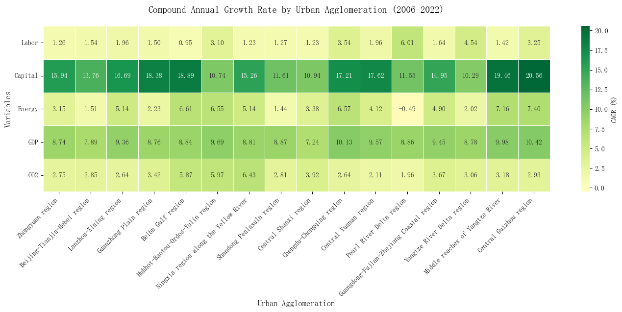
Figure 2. Compound annual growth rate by urban agglomeration (2006-2022)

The selection and computation of the above indicators are based on sound theoretical rationale, data availability, and model requirements. Table 1 presents descriptive statistics, and Fig. 2 illustrates the average annual growth rates of these input-output indicators for the 16 urban agglomerations. Overall, the data highlight clear differences in scale and characteristics across these urban agglomerations, with notable regional disparities emerging in both resource inputs and economic outputs.

In terms of inputs, the Pearl River Delta region shows the fastest labor growth (6.01%), while the Beibu Gulf region exhibits the slowest growth (0.95%), potentially reflecting the strong economic attractiveness and population inflows in the Pearl River Delta, as well as unbalanced labor and employment growth among regions. Meanwhile, Central Guizhou shows the highest growth rate in capital stock (20.56%), far exceeding that of more developed regions like the Yangtze River Delta (10.29%), likely due to rapid capital accumulation in these latecomer areas. Additionally, regional energy consumption growth varies considerably, with the Beibu Gulf region registering the fastest increase (6.61%) and the Pearl River Delta region showing a slight decline (-0.49%), likely driven by successful industrial upgrading and energy-saving policies. From an economic perspective, Central Guizhou also exhibits the highest GDP growth (10.42%), while Central Shanxi reports the lowest (7.24%), indicating diverging regional economic growth rates. Environmentally, the Ningxia region along the Yellow River records the fastest rise in CO₂ emissions (6.43%), substantially outpacing other regions, while the Pearl River Delta shows the lowest increase (1.96%), reflecting a focus on environmental protection and sustainable development amid economic expansion. These findings provide strong empirical support for subsequent analyses of the carbon emission efficiency of various urban agglomerations and inform regionally differentiated governance strategies.

4. Empirical analysis

4.1. Carbon emission efficiency index analysis

Using panel data from China’s 16 national-level urban agglomerations over 2006–2022, this study applies the Non-Radial Directional Distance Function (NDDF) approach alongside the Global Malmquist-Luenberger (GML) index. Specifically, the Carbon Reduction Efficiency Index (CREI) focuses on single-period performance in emission reduction and output, while the GML index tracks intertemporal changes, thereby ensuring both logical rigor and dual perspectives—short term and long term—for comprehensive explanatory power. Through linear programming, we evaluate static efficiency levels at both the national scale and across each urban agglomeration, then further decompose the dynamic changes in productivity, revealing the respective contributions of efficiency improvement and technological progress. These results offer empirical evidence for analyzing the spatial distribution and temporal evolution of carbon emission performance among urban agglomerations.

4.1.1. Annual performance analysis

According to Table 2, the CREI values of the selected urban agglomerations exhibit significant disparities during the study period, indicating pronounced differences in efficiency relative to the production frontier. The Pearl River Delta region consistently records a CREI of 1.000, reflecting its position at the technological frontier and maximization of carbon reduction potential. Shandong Peninsula region and Huhhot-Baotou-Ordos-Yulin region both reach CREI = 1.000 from 2009 onward, remaining stable and showing notable efficiency gains. In contrast, the CREI of Ningxia region along the Yellow River declines from 0.093 in 2006 to 0.046 in 2022, and Central Shanxi region drops from 0.181 to 0.105, both remaining at relatively low levels; the Chengdu-Chongqing region and the Beibu Gulf region display clear signs of efficiency deterioration. These differences mainly stem from variations in industrial structure, policy enforcement, and technological capacity across urban agglomerations.

Table 2. Carbon emission reduction efficiency index for urban agglomeration (2006-2022)

Referring to Fig. 3, the box plots visually depict the distribution of the carbon reduction efficiency index for each agglomeration. The length of each box represents the interquartile range (i.e., the middle 50% of the data), and the upper and lower edges indicate data boundaries. Shorter boxes, such as in the Beijing-Tianjin-Hebei region, suggest relatively concentrated annual carbon emission performance with minimal volatility. By contrast, longer boxes for agglomerations such as the Beibu Gulf region and the Middle Reaches of the Yangtze River region underscore large inter-annual variation in carbon reduction efficiency.

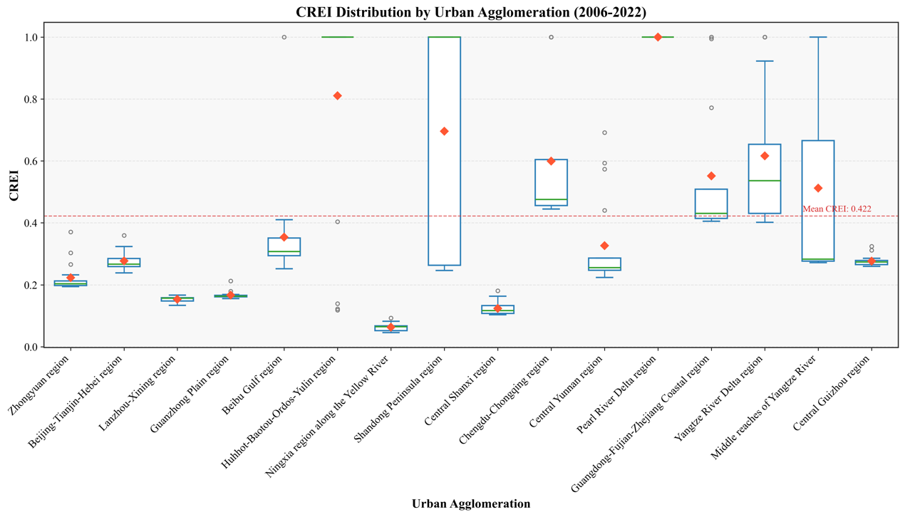
Figure 3. CREI distribution by urban agglomeration (2006-2022)

From a developmental perspective, regions like the Pearl River Delta region and the Yangtze River Delta region may benefit from advanced industrial structures—particularly high-tech manufacturing and modern services—leading to high energy efficiency and stable carbon emission performance. In contrast, regions such as Ningxia region along the Yellow River and Central Shanxi region primarily rely on traditional, high-energy-consuming industries, which, though supporting economic growth, confront significant carbon reduction pressures that hamper performance. Urban agglomerations exhibiting considerable performance volatility may be undergoing industrial transitions whose annual outcomes and policy implementations vary, thereby causing greater fluctuations in efficiency.

4.1.2. Temporal trends and regional comparisons

Over different years, the carbon reduction efficiency (CREI) of the 16 urban agglomerations shows notable changes, reflecting the progressive realization of national low-carbon policies.

When viewed over time, the CREI of several urban agglomerations exhibits diverging trajectories. Some regions show sustained growth, such as the Central Yunnan region (increasing from 0.287 to 0.692 at an average annual growth rate of 5.66%) and the Yangtze River Delta region (from 0.508 to 1.000 at 4.33%). Others, such as the Beibu Gulf region (from 1.000 to 0.252, averaging -8.26% per year) and the Beijing-Tianjin-Hebei region (from 0.359 to 0.289, averaging -1.36%), experience marked declines. A comparison across regions reveals significantly higher average CREI in eastern urban agglomerations compared to mid-western ones (e.g., Ningxia region along the Yellow River at 0.063, Central Shanxi region at 0.123), highlighting distinct regional heterogeneity. Notably, the Huhhot-Baotou-Ordos-Yulin region, though located in China’s mid-west, has maintained a CREI of 1.000 since 2009, suggesting efficiency levels on par with those of eastern clusters.

4.1.3. Overall Gini coefficient analysis

Lastly, Fig. 4 provides an overview of the overall Gini coefficient for carbon reduction efficiency. A comparative assessment of the coefficient time series against average CREI data indicates a strong association. From 2006 to 2019, while the carbon emission performance average fluctuated within 0.36–0.45, the Gini coefficient also remained relatively high and unstable, reflecting substantial performance disparities among urban agglomerations. Around 2008, in the wake of the global financial crisis, the average carbon reduction performance declined while the Gini coefficient rose, illustrating the differentiated impacts of economic shocks on clusters at distinct development stages; those with higher reliance on traditional industries faced stagnation or reversal in carbon reduction efforts, whereas mature regions—drawing on more advanced industrial structures and stronger technology—maintained relatively stable carbon emissions, thereby widening the gap.

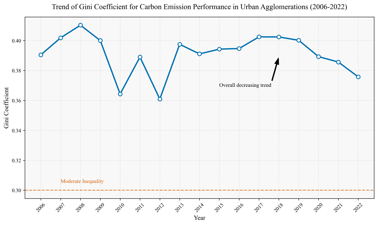
Figure 4. Trend of Dagum’s Gini coefficient for carbon emission performance in urban agglomerations (2006-2022)

After 2020, a series of unified reduction policies aligned with the carbon peaking and the carbon neutrality goalssubstantially elevated carbon reduction efficiency in lower-performing agglomerations, raising the average CREI to 0.51 or higher and driving down the Gini coefficient. The improved policy support, technology guidance, and funding resources granted to lower-performing agglomerations enable them to catch up with advanced regions, promoting more balanced regional development.

4.1.4. Efficiency evaluation

The differing CREI outcomes stem from three principal factors. First, industrial structure exerts a decisive influence: the Pearl River Delta region and the Yangtze River Delta region attain high CREI partly due to robust tertiary sectors and higher energy efficiencies. Second, policy effects are notable: the implementation of energy conservation and emission reduction measures has propelled some urban agglomerations to rapidly increase CREI, and the carbon peaking and the carbon neutrality goals introduced in 2020 further accelerated efficiency improvements. Technological advances and resource endowments also shape regional disparities; eastern agglomerations benefit from technology-driven improvements in efficiency, whereas midwestern agglomerations remain constrained by traditional industrial structures. These findings underscore the necessity of designing differentiated low-carbon development policies. The following analysis employs the GML index in a global NDDF framework to further examine intertemporal changes, providing more precise policy recommendations for low-carbon transitions among urban agglomerations.

4.2. Dynamic analysis of carbon emission performance

To comprehensively evaluate changes in carbon emission performance among China’s 16 national-level urban agglomerations from 2006 to 2022, this study employs the GML index and its decomposition method. The analysis captures trends in Total Factor Carbon Emission Productivity (TFCEP), subsequently separated into Efficiency Change (EC) and Technological Change (TC).

4.2.1. Overall trend analysis

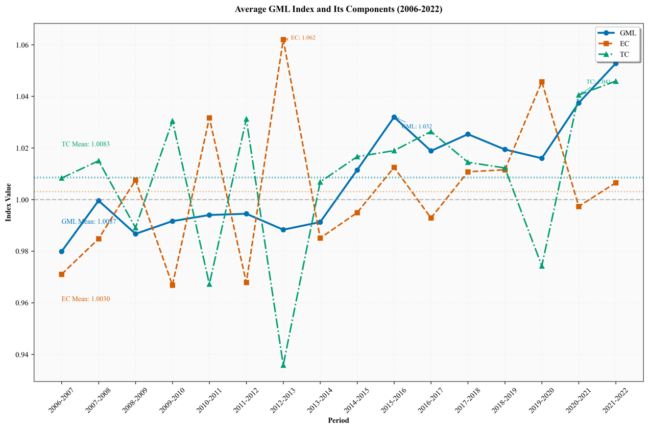
Figure 5. Trends in the average urban agglomerations (2006-2022)

As demonstrated in Fig. 5 and Table 3 the carbon emission performance of the 16 urban agglomerations fluctuates over the 2006–2022 period, with the average GML index slightly exceeding 1.000, indicating incremental overall improvements. For example, the GML of the Zhongyuan region increased from 0.994 (<1.000) in 2006–2007 to 1.047 (>1.000) in 2021–2022, showing a noticeable upward trend. In the early phase (2006–2010), several urban agglomerations had GML values below 1.000, such as the Guanzhong Plain region (0.974 in 2006–2007) and the Beibu Gulf region (0.735 in the same period). However, in the later period (2015–2022), GML values approached or exceeded 1.000. For instance, the Yangtze River Delta region reached 1.119 in 2020–2021, and the Guangdong-Fujian-Zhejiang Coastal region achieved 1.132 in 2021–2022. This trend suggests that the deepening of low-carbon policies and ongoing economic restructuring in China have contributed to improvements in carbon emission performance, particularly after the introduction of the "the carbon peaking and the carbon neutrality goals goals in 2020. However, there were some years where GML values fell below 1.000 (e.g., 0.735 for the Beibu Gulf region in 2006–2007 and 0.944 for the Central Guizhou region in 2012–2013), reflecting setbacks and the complexity of dynamic changes.

Table 3. GML of urban agglomerations (2006-2022)

4.2.2. Differences across urban agglomerations

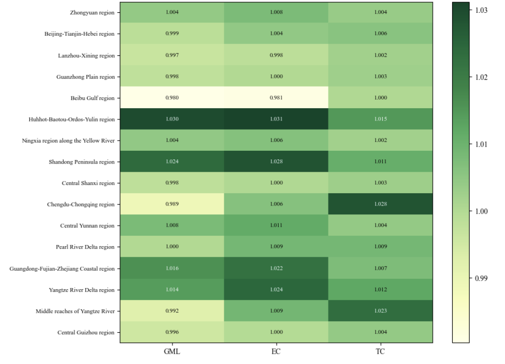
Figure 6. Heat map of the average index for urban agglomerations (2006-2022)

The GML index reveals significant heterogeneity among urban agglomerations, highlighting a geographically differentiated pattern of carbon emission performance. The Pearl River Delta region shows relatively high GML values from 2006 to 2008, but experiences a decline to 0.971 between 2019 and 2020, suggesting some volatility. Notably, the region steadily approaches the global frontier, as indicated by its rising EC values, which consistently approach 1.000. This suggests that variations in performance are primarily driven by technological change (TC). In contrast, the Huhhot-Baotou-Ordos-Yulin region saw a substantial increase in its GML, reaching 1.245 in 2021–2022. This significant rise, marked by a TC value of 1.245, well above the EC value of 1.000, underscores the crucial role of technological advancements in improving performance. On the other hand, the Beibu Gulf region exhibited a relatively low GML of 0.735 in 2006–2007, with both EC (0.772) and TC (0.952) below 1.000, indicating stagnant efficiency and technological progress. Spatially, mid-western agglomerations such as the Ningxia region along the Yellow River have lower GML values (0.858 in 2013–2014), while eastern regions, such as the Yangtze River Delta and the Guangdong-Fujian-Zhejiang Coastal region, show GML values exceeding 1.000 in later years (e.g., 1.075 for the Yangtze River Delta in 2021–2022), reflecting escalating disparities between regions. These variations can be attributed to differing levels of economic development, industrial restructuring, and technological innovation. Fig. 6 provides a visual representation of the average values of three key indices across all urban agglomerations.

4.2.3. Analysis of driving factors

The decomposition of the GML index reveals that Efficiency Change (EC) and Technological Change (TC) have distinct impacts on carbon emission performance across different urban agglomerations and time periods. For example, in the Zhongyuan region, the GML was 0.980 in 2012–2013, with an EC of 1.038 (>1.000), indicating substantial “catch-up” efficiency. However, the TC was 0.945 (<1.000), suggesting that technical regression partially offset the efficiency gains. By 2017–2018, the GML increased to 1.073, with both EC (1.055) and TC (1.017) exceeding 1.000, showing that both efficiency and technology played a role in performance improvements. In the Huhhot-Baotou-Ordos-Yulin region, the GML in 2008–2009 was 1.019, driven by an EC of 1.421, indicating significant “catch-up” efficiency. However, the TC was only 0.717, indicating that the production frontier itself had regressed. In the Beibu Gulf region (2006–2007), the GML was 0.735, with both EC (0.772) and TC (0.952) below 1.000, signaling that neither efficiency nor technology met expectations.

In contrast, in eastern regions like the Yangtze River Delta and the Guangdong-Fujian-Zhejiang coastal region, the GML showed an upward trend. In the Yangtze River Delta, the GML reached 1.022 in 2015–2016, primarily driven by EC (1.047). Similarly, in the Guangdong-Fujian-Zhejiang coastal region, the GML reached 1.144 in 2019–2020, largely influenced by EC (1.172). These findings suggest that “catch-up” efficiency is a key driver of short-term carbon emission performance improvement in certain regions (e.g., Huhhot-Baotou-Ordos-Yulin and Zhongyuan regions), while technological progress is more critical for long-term sustainability in advanced eastern regions such as the Pearl River Delta and the Yangtze River Delta. Consequently, this analysis provides valuable insights for designing region-specific low-carbon strategies: central and western agglomerations should prioritize enhancing efficiency, while eastern regions should focus on fostering technological innovation to sustain carbon emission performance improvements.

4.2.4. Performance evaluation

Analysis of the GML index for China’s 16 national-level urban agglomerations between 2006 and 2022 reveals an overall positive yet notably volatile trajectory in carbon emission performance. Spatially, the eastern agglomerations (e.g., Pearl River Delta region, Yangtze River Delta region) continue to lead in efficiency and technological innovation, whereas mid-western ones (e.g., Ningxia region along the Yellow River, Beibu Gulf region) exhibit greater instability. Decomposition of the GML index underscores significant spatiotemporal heterogeneity in the contributions of efficiency catch-up (EC) and technological progress (TC). This variation likely arises from differing policy incentives, degrees of industrial restructuring, and innovation capacities across regions. Specifically, mid-western clusters should emphasize technology introduction and transfer, optimizing industrial structures and elevating the level of technological transformation, whereas eastern clusters ought to consolidate their innovation advantages and steer efficiency toward the global frontier to achieve coordinated, low-carbon development goals at a regional scale.

5. Conclusion

Economic restructuring and technological advancement are pivotal pathways for improving carbon emission performance in urban agglomerations and facilitating China’s regional low-carbon transition. This study systematically evaluates the carbon emission performance of 16 national-level urban agglomerations in China from 2006 to 2022 using a Non-Radial Directional Distance Function and the Global Malmquist-Luenberger (GML) index. The results highlight significant regional heterogeneity and periodic variation in carbon emission performance. Eastern "optimization-enhancing" urban agglomerations, such as the Pearl River Delta and Yangtze River Delta regions, have long been at the technological frontier, exhibiting consistently high performance. In contrast, central and western "development-nurturing" and "growth-enhancing" urban agglomerations display relatively lower performance, though they possess considerable potential for improvement. Furthermore, the decomposition of the GML index reveals that the continuous advances in the eastern regions are primarily driven by long-term, stable technological progress (TC), while central and western regions rely more on efficiency improvements (EC) to close the performance gap. This finding enriches the theoretical framework of regional low-carbon development and provides new insights into the dynamic mechanisms of carbon reduction across China’s urban agglomerations.

Based on these findings, carbon reduction strategies should be tailored to the specific needs of different urban agglomerations, emphasizing the synergy between efficiency improvements and technological progress. For "optimization-enhancing" and "growth-enhancing" clusters, leveraging technological innovation is crucial. This involves guiding industrial structures toward higher-level green and low-carbon paradigms, solidifying the first-mover advantage in regional development. Additionally, investing more in research and development (R&D) of green technologies and establishing a robust carbon emissions trading system can direct resources to more efficient, low-carbon industries. For "development-nurturing" clusters, the focus should be on exploiting efficiency-based catch-up potential, accelerating the transition away from energy- and emissions-intensive industries, and reducing the costs of industrial restructuring through green finance and targeted policy support. This approach can facilitate leapfrogging toward low-carbon development.

On the regional coordination front, it is essential to establish cross-regional collaboration mechanisms that promote the diffusion and sharing of advanced low-carbon technologies, as well as a unified system for carbon emission monitoring and evaluation. This will create a lasting framework for collaborative emission reduction. Moreover, government agencies should strengthen top-level design, refine the fiscal transfer payment system, and provide more robust policy and financial support for the low-carbon transition in central and western regions. This would help reduce disparities in carbon reduction capacity nationwide, fostering more balanced and sustainable development across the country.

Finally, several limitations remain in this study. First, due to the quality and availability of statistical data, there may be inaccuracies in estimating carbon emissions within urban agglomerations. Second, the NDDF approach is sensitive to outliers and does not fully account for spatial spillover effects or policy interactions among different agglomerations. Future research could improve upon these limitations by (1) integrating multiple data sources and enhancing data quality to construct a more comprehensive database of urban agglomeration carbon emissions, (2) applying spatial econometrics or machine learning techniques to more accurately identify the drivers and spatial interaction mechanisms of carbon emission performance, and (3) refining the research scale by extending analyses to municipal and enterprise levels. This would establish a multi-scale analytical framework and provide more precise scientific evidence for low-carbon policymaking at various levels. Such enhancements would deepen the understanding of China’s regional low-carbon transition pathways and offer stronger theoretical and practical guidance for achieving the nation’s carbon peaking and carbon neutrality goals.

References

[1]. Wang, Q., Wang, X., Li, R., et al. (2024). Reinvestigating the environmental Kuznets curve (EKC) of carbon emissions and ecological footprint in 147 countries: a matter of trade protectionism. Humanities and Social Sciences Communications, 11(1), 160.
[2]. Cheng, J., Yi, J., Dai, S., et al. (2019). Can low-carbon city construction facilitate green growth? Evidence from China's pilot low-carbon city initiative. Journal of Cleaner Production, 231, 1158-1170.
[3]. Wang, S., Wang, Z., Fang, C. (2021). Evolutionary characteristics and driving factors of carbon emission performance at the city level in China. Science China (Earth Sciences), 65(7), 1292-1307.
[4]. Yu, T., Shu, T., Xu, J. (2019). Spatial pattern, and evolution of China’s urban agglomerations. Frontiers of Urban and Rural Planning, 2(1), 7.
[5]. Ang, B. W. (1998). Is the energy intensity a less useful indicator than the carbon factor in the study of climate change? Energy Policy, 27(15), 943-946.
[6]. Mielnik, O., Goldemberg, J. (1999). Communication The evolution of the “carbonization index” in developing countries. Energy Policy, 27(5), 307-308.
[7]. Sun, J. W. (2005). The decrease of CO2 emission intensity is decarbonization at national and global levels. Energy Policy, 33(8), 975-978.
[8]. Färe, R., Grosskopf, S., Norris, M. (1994). Productivity growth, technical progress, and efficiency change in industrialized countries. American Economic Review, 84(1), 66-83.
[9]. Charnes, A., Cooper, W. W., Rhodes, E. (1978). Measuring the efficiency of decision making units. European Journal of Operational Research, 2(6), 429-444.
[10]. Banker, R. D., Charnes, A., Cooper, W. W. (1984). Some Models for Estimating Technical and Scale Inefficiencies in Data Envelopment Analysis. Management Science, 30(9), 1078-1092.
[11]. Färe, R., Grosskopf, S. (2010). Directional distance functions and slacks-based measures of efficiency. European Journal of Operational Research, 200(1), 320-322.
[12]. Zhou, P., Ang, B. W., Wang, H. (2012). Energy and CO2 emission performance in electricity generation: A non-radial directional distance function approach. European Journal of Operational Research, 221(3), 625-635.
[13]. Zhang, H., Feng, C., Zhou, X. (2020). Going carbon-neutral in China: Does the low-carbon city pilot policy improve carbon emission efficiency? Sustainable Production and Consumption, 33, 312-329.
[14]. Färe, R., Grosskopf, S., Tyteca, D. (1996). An activity analysis model of the environmental performance of firms—application to fossil-fuel-fired electric utilities. Ecological Economics, 18(2), 161-175.
[15]. Färe, R., Grosskopf, S., Pasurka, C. A. (2007). Environmental production functions and environmental directional distance functions. Energy, 32(7), 1055-1066.
[16]. Dong, F., Li, X., Long, R. (2013). Regional carbon emission performance in China according to a stochastic frontier model. Renewable and Sustainable Energy Reviews, 28, 525-530.
[17]. Zhou, P., Delmas, M. A., Kohli, A. (2017). Constructing meaningful environmental indices: A nonparametric frontier approach. Journal of Environmental Economics and Management, 85, 21-34.
[18]. Chambers, R. G., Chung, Y., Färe, R. (1996). Benefit and distance functions. J Econ Theory, 70(2), 407-419.
[19]. Shao, S., Fan, M., Lili, Y. (2021). Economic Restructuring, Green Technical Progress, and Low-Carbon Transition Development in China: An Empirical Investigation Based on the Overall Technology Frontier and Spatial Spillover Effect. Journal of Management World, 38(2), 46-69+4-10.
[20]. Zhang, N., Zhou, P., Choi, Y. (2013). Energy efficiency, CO2 emission performance and technology gaps in fossil fuel electricity generation in Korea: A meta-frontier non-radial directional distance function analysis. Energy Policy, 56, 653-662.
[21]. Chung, Y. H., Färe, R., Grosskopf, S. (1997). Productivity and Undesirable Outputs: A Directional Distance Function Approach. Journal of Environmental Management, 51(3), 229-240.
[22]. Oh, D.-H. (2010). A global Malmquist-Luenberger productivity index. Journal of Productivity Analysis, 34(3), 183-197.
[23]. Zhang, N., Choi, Y. (2013). Total-factor carbon emission performance of fossil fuel power plants in China: A metafrontier non-radial Malmquist index analysis. Energy Economics, 40, 549-559.
[24]. Wang, Z., Feng, C. (2015). Sources of production inefficiency and productivity growth in China: A global data envelopment analysis. Energy Economics, 49, 380-389.
[25]. Du, J., Chen, Y., Huang, Y. (2018). A Modified Malmquist-Luenberger Productivity Index: Assessing Environmental Productivity Performance in China. European Journal of Operational Research, 269(1), 171-187.
[26]. Zhang, N., Kong, F., Choi, Y. (2016). The effect of size-control policy on unified energy and carbon efficiency for Chinese fossil fuel power plants. Energy Policy, 70, 193-200.
[27]. Dagum, C. (1997). A new approach to the decomposition of the Gini income inequality ratio. Empirical Economics, 22(4), 515-531.
[28]. Shan, H. (2008). Reestimating the Capital Stock of China: 1952~2006. Journal of Quantitative & Technological Economics, 25(10), 17-31.
[29]. Wu, Y., Shi, K., Chen, Z. (2023). Developing Improved Time-Series DMSP-OLS-Like Data (1992–2019) in China by Integrating DMSP-OLS and SNPP-VIIRS. IEEE Transactions on Geoscience and Remote Sensing, 60, 1-14.
[30]. Wang, S., Fang, C., Sun, L. (2019). Decarbonizing China’s Urban Agglomerations. Annals of the American Association of Geographers, 109(1), 266-285.
[31]. Commission, E., Centre, J. R., Crippa, M., et al. (2022). GHG emissions of all world countries. Publications Office of the European Union.
Cite this article
Zhuang,R. (2025). Measuring and analyzing carbon emission performance of Chinese national urban agglomerations: a static-dynamic integrated approach based on NDDF-GML. Journal of Applied Economics and Policy Studies,18(2),61-76.
Data availability
The datasets used and/or analyzed during the current study will be available from the authors upon reasonable request.
Disclaimer/Publisher's Note
The statements, opinions and data contained in all publications are solely those of the individual author(s) and contributor(s) and not of EWA Publishing and/or the editor(s). EWA Publishing and/or the editor(s) disclaim responsibility for any injury to people or property resulting from any ideas, methods, instructions or products referred to in the content.
About volume
Journal:Journal of Applied Economics and Policy Studies
© 2024 by the author(s). Licensee EWA Publishing, Oxford, UK. This article is an open access article distributed under the terms and
conditions of the Creative Commons Attribution (CC BY) license. Authors who
publish this series agree to the following terms:
1. Authors retain copyright and grant the series right of first publication with the work simultaneously licensed under a Creative Commons
Attribution License that allows others to share the work with an acknowledgment of the work's authorship and initial publication in this
series.
2. Authors are able to enter into separate, additional contractual arrangements for the non-exclusive distribution of the series's published
version of the work (e.g., post it to an institutional repository or publish it in a book), with an acknowledgment of its initial
publication in this series.
3. Authors are permitted and encouraged to post their work online (e.g., in institutional repositories or on their website) prior to and
during the submission process, as it can lead to productive exchanges, as well as earlier and greater citation of published work (See
Open access policy for details).