1. Introduction

Nowadays, identifying a beneficial portfolio attracts extraordinary attention, particularly in the context of increasingly volatile financial markets and diverse investment instruments. Joemon et al. [1] state that with the goal of optimizing returns while reducing risk exposure, portfolio diversification requires striking a balance between expected returns and return variance, as proposed by Modern Portfolio Theory (Markowitz, 1952). Prior to Markowitz's groundbreaking research, qualitative judgment was primarily used when making investment decisions. This was completely changed by the introduction of Modern Portfolio Theory (MPT), which established the concepts of diversification and risk-return optimization. MPT not only solidifies its role as the cornerstone of contemporary financial economics but also propels decades of groundbreaking theoretical and empirical advancements in the field, furthermore, extending its principles to diverse domains. For instance, its incorporation into programming serves as the foundation for algorithmic risk management solutions [2]. Additionally, MPT's cross-sector applications show how adaptable it is in tackling long-term capital allocation problems, like maximizing risk diversification in real estate through asset type and geographic allocations [3]. These illustrations show that MPT research and optimization are still crucial and beneficial today, especially for improving quantitative approaches and solving realistic resource allocation issues.

Although the theoretical framework is well-established, there are several barriers to practical implementation, including (1) matrix invertibility is compromised by the covariance matrices' singularity under practical asset correlations; (2) the contradiction between real-world short-selling limits and theoretical presumptions of unlimited short-selling; and (3) inadequate consideration of risk-free assets within frameworks for portfolio optimization. This paper addresses these challenges with mathematical frameworks like symmetric matrix optimization, iterative weight elimination algorithms, and dynamic threshold analysis to balance practical circumstances with theoretical rigor. Furthermore, using historical data from twelve actual stocks offers actionable insights toward optimizing a portfolio under realistic limitations.

To analyze portfolio optimization, this study gives two cases: (1) portfolios comprising exclusively risky assets, and (2) portfolios incorporating risk-free assets. This is addressed by setting up a condition-driven equality-constrained optimization problem and then solving it with the Lagrange multiplier method. Four parts will be discussed in the rest of paper: (1) modeling extremum problems using idealized assumptions. (2) To identify effective frontier solutions, the Mean-Variance Optimization (MVO) model is consulted and improved. (3) Analyzing risk-return preferences with frontier graphics. (4) extending the framework by adding a risk-free asset and analyzing market-contingent portfolio strategies.

2. Literature review

By establishing a mathematical framework for optimizing portfolio allocation by maximizing returns for a given level of risk, Modern Portfolio Theory (MPT), which was developed in the middle of the 20th century, completely changed how investors thought about the tradeoff between risk and return [4]. This theory is based on two fundamental assumptions: first, that asset returns are distributed normally, and second, that diversification may effectively reduce risk. MPT, which initially was created for the financial markets, makes it possible to build a portfolio of financial assets [5]. A portfolio is an assortment of financial assets that are combined and rearranged to satisfy an investor's aims. Each investor's primary goal when building a portfolio is to minimize risk and maximize return [6]. The main benefit of creating such a portfolio is that it promotes diversification, which evens out the equity curve and yields a higher return per risk than trading individual assets [7]. Risk and return are the most critical elements for the construction of a portfolio. In this study, if a portfolio has the least amount of volatility among those with the same projected rate of return, it is considered a frontier portfolio. The efficient frontier consists of portfolios with positive returns located above the Minimum Variance Portfolio (MVP) point, where MVP represents the portfolio with the lowest achievable risk. This study extends previous work by showing that when a risk-free asset is included, the efficient frontier becomes a linear Capital Market Line (CML). Therefore, this extension aligns the theoretical framework with actual market dynamics and enables investors to achieve superior risk-return trade-offs.

Markowitz (1952) defined the expected return of a portfolio as the weighted average expected return of each of the assets that make up the portfolio. The covariance between the returns of every pair in a portfolio affects its risk (as indicated by standard deviation), in addition to the risk of its individual assets [8]. A lot of information in the Markowitz Model needs to be estimated. Chakraborty and Patel [9] reveal that W.E. Sharpe therefore created a new and more straightforward model to analyze the portfolio in 1964. This concept states that the return on an asset is linked to a single index, typically a market index. The market index will include all equities traded on the exchange. In line with the hypothesis by previous research, the theoretical basis for the combination of a risk-free asset is further clarified in this paper, proving that the conventional hyperbolic efficient frontier becomes a linear Capital Market Line (CML). This change brings in the tangency portfolio, a crucial invention that helps investors attain higher risk-return trade-offs in a range of market circumstances.

3. Key concepts and theoretical foundations

3.1. Markowitz mean-variance optimization model

3.1.1. Model assumptions

Markowitz (1952) developed the mean-variance optimization paradigm, which quantifies the tradeoff between risk (variance of returns) and predicted return and serves as a foundation for portfolio selection. To thoroughly identify the efficient frontier—the collection of portfolios that deliver the highest return for certain levels of risk, this study makes three idealized assumptions.

(1) Frictionless markets: no transaction costs and unlimited short selling.

(2) Non-singular variance-covariance matrix: Ensuring invertibility for computational feasibility.

(3) Normally distributed returns: Simplifying risk modeling despite empirical deviations.

3.1.2. Formulation of the optimization problem

The portfolio with the lowest variability among all the portfolios with an identical expected return is called a frontier portfolio. This is expressed mathematically as a constrained optimization problem (see formula 1):

\( _{\lbrace w\rbrace }^{min} \frac{1}{2}{w^{T}}Vw \) (1)

Subject to: \( {w^{T}}e=E[{\widetilde{r}_{p}}] \) and \( { w^{T}}1=1 \)

Let p represent a frontier portfolio, w denotes the N-vector portfolio weights of p. V stands for the variance-covariance matrix of asset returns. e defines the vector of expected returns on the N risky assets. \( E[{\widetilde{r}_{p}}] \) denotes the target portfolio return and 1 is the unit vector.

We use the Lagrange multipliers λ and γ to solve this limited optimization, which turns the problem into an unconstrained formula (2):

\( _{\lbrace w,λ,γ\rbrace }^{ min} L= \frac{1}{2}{w^{T}}Vw+λ(E[{r_{p}}]-{w^{T}}e)+γ(1-{w^{T}}1) \) (2)

Taking partial derivatives of L with respect to \( w, λ, and γ, \) we derive a system of N+2 linear equations. Solving this system using Cramer's rule yields the following constants formula (3)-(6):

\( {A=1^{T}}{V^{-1}}e \) (3)

\( {B=e^{T}}{V^{-1}}e \) (4)

\( {C=1^{T}}{V^{-1}}1 \) (5)

\( D=BC-{A^{2}} \) (6)

The optimal portfolio weights are given by (see formula 7-9):

\( {w_{p}}=g+hE[{\widetilde{r}_{p}}] \) (7)

Where:

\( g=\frac{1}{D}[B({V^{-1}}1)-A({V^{-1}}e)] \) (8)

\( h=\frac{1}{D}[C({V^{-1}}e)-A({V^{-1}}1)] \) (9)

3.2. Mathematical representation of frontier portfolios

3.2.1. Derivation of portfolio weights

(1) Vector g: This vector represents the optimal portfolio weights when the expected portfolio return \( E[{\widetilde{r}_{p}}] \) is zero. Mathematically, it satisfies the budget constraint \( { g^{T}}1=1 \) , ensuring that the total investment allocation sums to unity. Conceptually, g serves as the baseline portfolio configuration under a risk-minimization objective without return targeting.

(2) Vector h: The vector h acts as a scaling factor that adjusts portfolio weights in proportion to the target expected return \( E[{\widetilde{r}_{p}}] \) . It satisfies \( { h^{T}}1=0 \) .

(3) Frontier Characterization: Any frontier portfolio can be uniquely expressed as a linear combination in Equation (7) of these vectors:

Equations (7) demonstrates that the entire set of efficient portfolios lies on the efficient frontier, a hyperbola in risk-return space. Conversely, all portfolios that fit this parametric description are necessarily frontier portfolios, thus a bijective relationship between target returns and ideal portfolio weights is established.

3.2.2. Covariance analysis of frontier portfolios

For any two frontier portfolios p and q, their return covariance is derived as equation (10):

\( {{Cov({\widetilde{r}_{p}},{\widetilde{r}_{q}})=w_{p}}^{T}}V{w_{q}}=\frac{C}{D}(E[{\widetilde{r}_{p}}]-A/C)(E[{\widetilde{r}_{q}}]-A/C) +1/C \) (10)

Where parameters A, B, C and D are defined in Equations (3)-(6).

Rearranging terms yields the variance expression for a single frontier portfolio p (see equation 11 and 12).

\( \frac{{σ^{2}}({\widetilde{r}_{p}})}{1/C} -\frac{{(E[{\widetilde{r}_{p}}]-A/C)^{2}}}{D/{C^{2}}}=1 \) (11)

\( {σ({\widetilde{r}_{p}})^{2}}=\frac{1}{D}{(C(E[{\widetilde{r}_{p}}])^{2}}-2AE[{\widetilde{r}_{p}}]+B) \) (12)

This equation describes a hyperbola in the risk-return space, with standard deviation σ ( \( \widetilde{r} \) ) as the horizontal axis and expected return E [ \( \widetilde{r} \) ​] as the vertical axis (Figure 1).

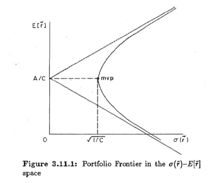
Figure 1. Portfolio frontier in the σ ( \( \widetilde{r} \) )-E [ \( \widetilde{r} \) ​] space

(1) Feasible Region: The feasible set of portfolios consists of the hyperbola and the region on its right side. All frontier portfolios lie exactly on the hyperbola, while suboptimal portfolios reside to the right.

(2) Minimum Variance Portfolio (MVP): The vertex of the hyperbola corresponds to the MVP, with coordinates: \( (\sqrt[]{1/C},A/C) \)

(3) Quadrant Analysis: Select an arbitrary point A within the feasible region, establish a Cartesian coordinate system with A as the origin, and carry out further analysis to assess portfolios' risk-return characteristics in comparison to A.

Quadrant II: Portfolios exhibit higher returns and lower risk than portfolio A, representing superior choices. Quadrant IV: Portfolios yield lower returns and higher risk, deemed inferior to A.

Quadrants I & III: Ambiguous dominance due to conflicting risk-return tradeoffs. This geometric approach provides sensitive insights into portfolio optimization strategies.

3.2.3. Effective and inefficient frontiers

The hyperbola bifurcates into two branches at the critical point \( E[{\widetilde{r}_{p}}] \) =A/C

(1) Upper Branch (Effective Frontier): This area is dominated by portfolios with positive returns. Investors seeking profit maximization focus exclusively on this branch.

(2) Lower Branch (Inefficient Frontier): Portfolios generate negative returns and for logical investors, portfolios are essentially meaningless.

3.2.4. Marginal risk-return tradeoff and sharpe ratio

(1) Marginal Risk-Return Tradeoff: Along the effective frontier, increasing the target return \( E[{\widetilde{r}_{p}}] \) ​ necessitates accepting incremental marginal risk. Formally, the marginal risk per unit return is given by equation (13):

\( \frac{∂σ{(\widetilde{r}_{p}})}{∂E[{\widetilde{r}_{p}}]}=\frac{CE[{\widetilde{r}_{p}}]-A}{Dσ{(\widetilde{r}_{p}})} \) (13)

This convex relationship implies risk-taking returns decrease as \( E[{\widetilde{r}_{p}}] \) increases.

(2) Investor Portfolio Optimization via Sharpe Ratio: The Sharpe ratio is a crucial psychological criterion for decision - making. It is the ratio of expected return to variance, which investors use when setting up investment portfolios. The optimal investment point is found where the Sharpe ratio line tangents the efficient frontier curve. This tangency point represents the portfolio that balances risk and expected gains to optimize risk-adjusted return.

The Sharpe ratio serves as a numerical indicator of risk attitudes among investors that separates risk-averse from risk-seeking behavior. Risk-seeking behavior encourages allocations toward portfolios with higher expected returns and Sharpe Ratios. Risk aversion causes a movement in preferences toward assets with reduced risk. The Minimum Variance Portfolio (MVP) is the extreme risk aversion. It reduces portfolio variance without considering return expectations.

4. Empirical analysis with real data

4.1. Data source and processing methods

As an example, this study employs the closing prices of twelve constituent stocks (ADM, BA, CAT, DE, GIS, GOOGL, HSY, IBM, JPM, MSFT, PG, WMT) across 61 trading days spanning 2011-2016 to perform computational analysis for deriving Efficient Frontier portfolio strategies.

4.2. Parameter calculation results

The daily closing prices of the 12 constituent stocks (ADM, BA, CAT, DE, GIS, GOOGL, HSY, IBM, JPM, MSFT, PG, WMT) were first converted into daily returns by the formula (14):

\( {R_{t}}=\frac{{P_{t}}-{P_{t-1}}}{{P_{t-1}}} \) (14)

Where \( {R_{t}} \) denotes the return on day t, and \( {P_{t}} \) denotes the closing price on day t.

The AVERAGE function in Excel was used to get the arithmetic mean of previous returns (see equation 15):

\( {μ_{t}}=\frac{1}{n}\sum _{t=1}^{n}({R_{t}}) \) (15)

The computed expected Returns are: 0.01037382; 0.015851847; 0.003536989; 0.005454629; 0.011749253; 0.018502757; 0.011681926; 0.000644734; 0.015450849; 0.017283281; 0.008708205; 0.007200771.

The VAR.P function in Excel was used to get the variance of previous returns (see equation 16):

\( σ_{t}^{2}=\frac{1}{n}\sum _{t=1}^{n}({{R_{t}}-{μ_{t}})^{2}} \) (16)

The computed variances are: 0.004061708; 0.003260351; 0.0047144; 0.002722354; 0.001689157; 0.003858339; 0.002599377; 0.00245572; 0.004644663; 0.004278525; 0.001467067; 0.002184394.

Using Equation (3), the following parameters were calculated: A=16.37633796, B=0.286554408, C=1762.267088, D=236.8009569

The vector g was derived as: [-0.035985486; -0.053072894; 0.088918614; 0.30046326; -0.062234704; 0.011189432; 0.093150975; 0.531478028; -0.254858703; -0.098428447; 0.359263833; 0.120116093].

The vector h was derived as: [5.012589574; 10.05671428; -5.401246776; -11.79992089; 17.1117234; 12.30548103; 1.604402092; -48.42679106; 23.25527376; 16.5214894; -28.73888364; 8.499168839].

The vector g satisfies the sum-to-unity constraint \( \sum g=1 \) , while the vector h adheres to the zero-sum condition \( \sum h=0 \) . Critical validation checks for computational consistency are provided by these properties.

4.3. Efficient frontier analysis

Given an expected return rate \( E[{\widetilde{r}_{p}}] \) ​, the optimal portfolio weights on the Efficient Frontier can be computed as: \( {w_{p}}=g+hE[{\widetilde{r}_{p}}] \) by Equation (7)

Where: \( {w_{p}} \) denotes the vector of portfolio weights, g and h are precomputed by Equation (8)-(9).

As an illustrative case, when the expected return is set to \( E[{\widetilde{r}_{p}}] \) =0.01, the computed Efficient Frontier portfolio weights derived are:

\( {w_{p}} \) = [0.01414041; 0.047494249; 0.034906146; 0.182464051; 0.10888253; 0.134244242; 0.109194996; 0.047210117; -0.022305965; 0.066786447; 0.071874996; 0.205107781]

Notably, one component exhibits a negative weight \( {w_{9}}=-0.022305965 \) , which represents a short position in the corresponding asset. The treatment of short-selling limits in portfolio optimization must be discussed in consideration of this.

4.4. Weight adjustment under short-selling constraints

(1) To eliminate short - selling positions, assets with negative weights are iteratively eliminated from the portfolio. The leftover assets are then used to re-optimize the portfolio. Until all asset weights comply with the non-negative condition, this process is repeated (see formula 17):

\( {w_{i}}≥0 ∀I \) (17)

This sequential exclusion guarantees that the final solution adheres to no-short-selling limitations.

(2) Handling Weights Exceeding Unity (Leverage)

The presence of weights exceeding 1 is contingent upon the existence of negative weights in the unconstrained solution. By enforcing \( {w_{i}}≥0 \) , the necessity for compensatory long positions to offset hypothetical short sales is eliminated, thereby inherently bounding all weights within formula (18):

\( 0≤{w_{j}}≤1 ∀j \) (18)

(3) Following the elimination of the negative-weighted asset, we recompute the Efficient Frontier solution using the reduced universe of 11 component stocks. The optimized portfolio weights are listed by the parameter vector:

\( {w_{p}} \) = [0.014665321; 0.044350305; 0.039292786; 0.171658375; 0.10754829; 0.129208877; 0.10815592; 0.045183778; 0.056248357; 0.071417744; 0.212270248]

where all constituents satisfy \( {w_{i}}≥0 \) . The correctness of the limited optimization under non-negativity criteria is confirmed by this strictly positive weighting scheme. Thus, the Efficient Frontier's ultimately acceptable solution is established.

5. Portfolio optimization with risk-free asset

5.1. Extended optimization model

While the preceding analysis focused exclusively on N risky assets constructing the Efficient Frontier, we now extend the framework by introducing a riskless asset with return rate \( {r_{f}} \) .

New Equality-Constrained Optimization Problem is formulated as formula (19):

\( _{\lbrace w\rbrace }^{min} \frac{1}{2}{w^{T}}Vw \) (19)

subject to the equality constraint (see equation 20):

\( {w^{T}}e+(1-{w^{T}}1){r_{f}}=E[{\widetilde{r}_{p}}] \) (20)

Where \( {r_{f}} \) represents the risk-free rate of return. p denotes the frontier portfolio. w stands for the N-vector portfolio weights of p and V denotes the variance-covariance matrix of asset returns. e defines the vector of expected returns on the N risky assets. \( E[{\widetilde{r}_{p}}] \) defines the target portfolio return and 1 is the unit vector.

Following the use of the Lagrange multiplier method, the optimal weights are determined to be (see equation 21):

\( {w_{p}}={V^{-1}}(e-{r_{f}}1)\frac{E[{\widetilde{r}_{p}}]-{r_{f}}}{H} \) (21)

with constants defined as: \( {H=B-2A{r_{f}}+C{r_{f}}^{2}} \) (20). Where parameters A, B, C, and D are defined in Equations (3)-(6). Under the conditions \( {A^{2}}-BC \lt 0 and H \gt 0 \) , the solution is admissible. The portfolio return's variance is calculated as formula (22):

\( {σ^{2}}({\widetilde{r}_{p}})=\begin{cases} \begin{array}{c} \frac{E[{\widetilde{r}_{p}}] -{r_{f}}}{\sqrt[]{H}} if E[{\widetilde{r}_{p}}] ≥{r_{f}} \\ -\frac{E[{\widetilde{r}_{p}}] -{r_{f}}}{\sqrt[]{H}} if E[{\widetilde{r}_{p}}] \lt {r_{f}} \end{array} \end{cases} \) (22)

That is, two half-lines with slopes \( \sqrt[]{H} \) and - \( \sqrt[]{H} \) that originate from point \( {(0,r_{f}}) \) in the \( σ({\widetilde{r}_{p}})-E[{\widetilde{r}_{p}}] \) plane geometrically describe the portfolio frontier.

5.2. Frontier analysis under market conditions

To determine the intersection points between the half-lines and the hyperbola, it can be systematically categorized into three different cases. These cases result from the basic relationship between the parameters of the line and the inherent characteristics of the hyperbola.

5.2.1. Portfolio frontier under \( {r_{f}} \lt A/C \) (typical situation: advantageous market conditions) (figure 2)

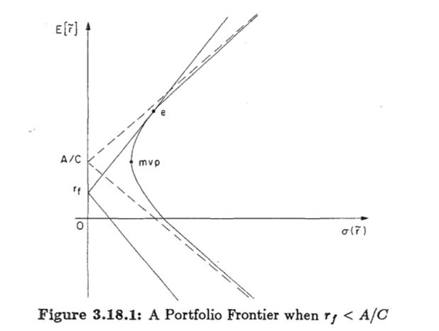
Figure 2. A portfolio frontier when \( {r_{f}} \lt A/C \)

A scenario displays efficient markets with a low risk-free rate relative to market risk-return trends. There is only one point of tangency shared by the two half-lines and the hyperbola. It is on the upper branch of the hyperbola called point \( {W_{e}} \) . Two critical portfolios should be noticed:

(1) Risk-free portfolio \( {(0, r_{f}}) \) : By allocating all resources to the risk-free asset, zero volatility is achieved.

(2) Market portfolio \( {W_{e}} \) : Fully invested in risky assets, reflecting pure market risk and return.

The frontier is divided into three distinct zones by the line connecting these two points:

(1) Infeasible regions: Region below and to the right of \( {(0, r_{f}}) \) implying short-selling risky assets (constrained by regulations). Region above and to the right of ​ \( {W_{e}} \) limiting by borrowing costs/margin requirements (leveraging)

(2) operationally feasible region:

This region lies strictly between \( {(0, r_{f}}) \) and \( {W_{e}} \) . A risk preference gradient can be apparent on the portfolio frontier: weights near \( {(0, r_{f}}) \) reflect conservative choices prioritizing capital preservation. Conversely, positions that approach \( {W_{e}} \) indicate a greater willingness to take risks to maximize returns. Empirical data supports This feasible portion is where rational investors primarily optimize, adjusting allocations to suit their utility preferences and risk tolerance.

5.2.2. Portfolio frontier under \( {r_{f}} \gt A/C \) (typical situation: adverse market conditions) (figure 3)

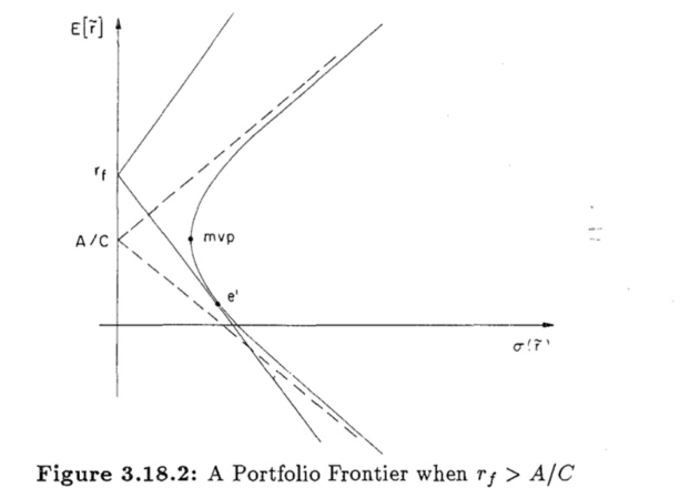
Figure 3. A portfolio frontier when \( {r_{f}} \gt A/C \)

A less frequent situation where the risk-free rate is higher than the market's risk-return ratio, signaling unfavorable market conditions. The hyperbola and two half-lines share a single tangency point, located on the lower branch (market as point e’).

Region below and to the right of e’ (leveraging) or above and to the right of ​ \( {(0, r_{f}}) \) (short-selling risky assets) are limited by financial or regulatory barriers.

operationally feasible region lies between e’ and \( {(0, r_{f}}) \) portfolios closer to e’ exhibit increasingly unfavorable risk-return profiles. The goal of rational investors is to move their holdings toward \( {(0, r_{f}}) \) by divesting risky assets. However, real-world obstacles like transaction fees or illiquid markets make these rebalancing exercises impractical.

5.2.3. Portfolio frontier under \( {r_{f}}=A/C \) (critical state) (figure 4)

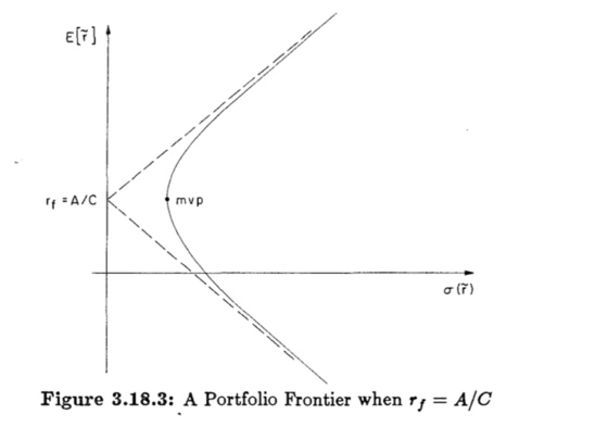
Figure 4. A portfolio frontier when \( {r_{f}}=A/C \)

Since the two half-lines in this case precisely correspond to the hyperbolics’ asymptote, there is no tangency point between risk-free and risky assets.

Considering financial markets are dynamic, this equilibrium situation is intrinsically unstable. The equality A gets disrupted by slight shifts in asset returns or risk-free rate adjustments, making this condition temporary and practically unobservable as an empirical standpoint.

6. Conclusion

To rigorously address risk-based portfolio optimization within the framework of Modern Portfolio Theory (MPT), this paper first develops an equality-constrained quadratic programming model under idealized assumptions. Then, through the Lagrange multiplier method and analytical derivations, we obtain solutions for frontier portfolios. By further visualizing these solutions, we present a clear geometric understanding of the Efficient Frontier and its relationship to diverse risk preferences. However, classical MPT frameworks have a practical limitation: negative weight allocations. Therefore, we propose a systematic methodology that iteratively refines portfolio constraints to eliminate such allocations. Through this approach, we bridge a critical gap between theoretical constructs and real-world implement ability. A 12-asset dataset is additionally utilized in this study to examine the theoretical framework in real-world scenarios. The whole mathematical procedure is thoroughly explained, with the computation of covariance matrices and the removal of negative weights. In this way, it blends strict methods with practical applications. This study makes two primary contributions: (1) Computational Refinement of Frontier Solutions: By simplifying improving the derivation of frontier portfolios and displaying their distribution on the risk-return plane, we provide an accessible geometric illustration of risk preferences. (2) Practical Extension with Risk-Free Assets: By incorporating a risk-free asset, we rigorously analyze its impact on portfolio optimization under real and comprehensive market conditions.

There are some limitations to this study, which could lead to further studies and recommendations for future directions: (1) Overly idealized assumptions: The model assumes frictionless markets and independent asset returns, but Real-world variables like transaction costs and asset correlations may generate discrepancies between theoretical and practical results. (2) Scalability and computational efficiency issues: For high-dimensional optimization problems, the Lagrange multiplier approach shows significant computational complexity. Large-scale asset portfolio scheduling is hampered by the possibility of mistakes caused by manual Excel computations. To bridge the gap between theoretical models and practical implementation, Future research should concentrate on incorporating real-world restrictions into equality-constrained optimization frameworks, such as asset interdependencies and transaction costs. In addition to reducing human error, developing specialized algorithms or software tools to automate computations will increase scalability for managing sizable and diverse portfolios. Subsequent research endeavors may investigate the multidisciplinary integration of this model with the desire to present fresh viewpoints and insights about portfolio optimization. focusing on the theoretical framework's applicability and practical relevance, such efforts may enhance its flexibility to meet changing investor needs and a diversity economic condition.

References

[1]. Joemon, B., Ghazanfar, M. A., Azam, M. A., Jhanjhi, N. Z., & Khan, A. A. (2023). Novel heuristics for Stock portfolio optimization using machine learning and Modern Portfolio Theory. 2023 International Conference on Business Analytics for Technology and Security (ICBATS), Business Analytics for Technology and Security (ICBATS), 2023 International Conference On, 1-6. https://doi.org/10.1109/ICBATS57792.2023.10111321
[2]. Dubach, P. (2022). A Python integration of practical asset allocation based on modern portfolio theory and its advancements.
[3]. Yang, R. (2011). Optimizing the Real Estate Portfolio Decision Model Based on Modern Portfolio Theory. 2011 Fourth International Joint Conference on Computational Sciences and Optimization, Computational Sciences and Optimization (CSO), 2011 Fourth International Joint Conference On, 1232–1235. https://doi-org-s.elink.xjtlu.edu.cn:443/10.1109/CSO.2011.195
[4]. Cinciulescu, D. (2024). The Impact of Tail Risk and Black Swan Events on Modern Portfolio Theory. A Reassessment of Risk Assumptions in Extreme Market Conditions. Young Economists Journal / Revista Tinerilor Economisti, 21(43), 83–96.
[5]. Silva Filho, M. C., Monteiro, C. C., Inácio, P. R. M., & Freire, M. M. (2024). A Distributed Virtual-Machine Placement and Migration Approach Based on Modern Portfolio Theory. Journal of Network and Systems Management, 32(1). https://doi-org-s.elink.xjtlu.edu.cn:443/10.1007/s10922-023-09775-8
[6]. V., J. B., & H. R., T. (2024). Construction of Optimum Portfolio Using Modern Portfolio Theory and Sharpe’s Single Index Model. Prajnān, 52(4), 335–351.
[7]. Ngo, V. M., Nguyen, H. H., & Van Nguyen, P. (2023). Does reinforcement learning outperform deep learning and traditional portfolio optimization models in frontier and developed financial markets? Research in International Business and Finance, 65. https://doi-org-s.elink.xjtlu.edu.cn:443/10.1016/j.ribaf.2023.101936
[8]. Maqbool, F., & Husnain, M. (2022). Optimising the Investor’s Portfolio through Modern Portfolio Theory: Empirical Evidence from Pakistan. NUML International Journal of Business & Management, 17(2), 1–15. https://doi-org-s.elink.xjtlu.edu.cn:443/10.52015/nijbm.v17i2.138
[9]. Chakraborty, S., & Patel, A. K. (2018). Construction of Optimal Portfolio Using Sharpe’s Single Index Model and Markowitz Model: An Empirical Study on Nifty 50 Stock. Journal of General Management Research, 5(1), 86–103.
Cite this article
Zhou,J. (2025). Construction of the efficient frontier for portfolios combining risky and risk-free assets: an MPT-Based optimization model and visualization analysis. Journal of Fintech and Business Analysis,2(2),1-9.
Data availability
The datasets used and/or analyzed during the current study will be available from the authors upon reasonable request.
Disclaimer/Publisher's Note
The statements, opinions and data contained in all publications are solely those of the individual author(s) and contributor(s) and not of EWA Publishing and/or the editor(s). EWA Publishing and/or the editor(s) disclaim responsibility for any injury to people or property resulting from any ideas, methods, instructions or products referred to in the content.
About volume
Journal:Journal of Fintech and Business Analysis
© 2024 by the author(s). Licensee EWA Publishing, Oxford, UK. This article is an open access article distributed under the terms and
conditions of the Creative Commons Attribution (CC BY) license. Authors who
publish this series agree to the following terms:
1. Authors retain copyright and grant the series right of first publication with the work simultaneously licensed under a Creative Commons
Attribution License that allows others to share the work with an acknowledgment of the work's authorship and initial publication in this
series.
2. Authors are able to enter into separate, additional contractual arrangements for the non-exclusive distribution of the series's published
version of the work (e.g., post it to an institutional repository or publish it in a book), with an acknowledgment of its initial
publication in this series.
3. Authors are permitted and encouraged to post their work online (e.g., in institutional repositories or on their website) prior to and
during the submission process, as it can lead to productive exchanges, as well as earlier and greater citation of published work (See
Open access policy for details).