1. Introduction

The most popular sport in the world is football, and the Fédération Internationale de Football Association (FIFA) hosts the World Cup every four years. With millions of spectators and billions in yearly income, this makes it the first sporting event ever [1]. Due to the intricacy and unpredictable nature of the game, forecasting the World Cup’s outcome has always been difficult. Machine learning techniques like the Gradient Boosting (GB) algorithm and RF algorithm have recently been used to forecast football games with a great degree of accuracy [2]. These algorithms have been applied to various football leagues and tournaments worldwide, including the English Premier League, La Liga and Serie A. Machine Learning (ML) can also help referees and FIFA to distinguish match-fixing situations [3]. However, predicting the outcome of the World Cup is still a challenging task due to the unique characteristics of this tournament. The World Cup is a knockout tournament where teams from different continents compete against each other. The teams’ performance in previous World Cups and their current form are essential factors that determine their chances of winning. Moreover, several other factors need to be considered when predicting the outcome of the World Cup, such as team composition, red card or yellow card, player injuries, weather conditions and home advantage [4].

Several studies have explored the use of ML methods to predict the outcome of sports events, including football games. A machine-learning algorithm was developed by a group of researchers from the Technical University of Munich, the Ghent University in Belgium, and the Technische Universität Dortmund in Germany to forecast potential World Cup winners in 2018 [5]. Another study trained a logistic regression model with data from previous World Cups to predict the winner of each World Cup match [6]. GB and Random Forest (RF) algorithms are widely used in ML and data science to make forecasts based on historical data. These algorithms have been used in multiple industries, including finance, economics, and sports. In recent years, there have been many technological developments in prediction work based on these algorithms. One example is the use of these algorithms to forecast real Gross Domestic Product (GDP) growth. In a report published in 2020, the two models were used to forecast Japan’s real GDP growth over the 17-year period from 2001. The study found that the forecasts made by these models were more accurate than the industry-standard estimates made by Japan’s own central bank and some international financial organisations [7].

With the help of GB and RF models, this study proposes a model for forecasting the World Cup results to address this problem. The proposed model is tested using a variety of performance metrics, including accuracy, precision, and more [8]. It is trained using historical data from prior World Cups. For football fans and analysts, the study’s findings offer useful information that will help them make highly accurate predictions about the World Cup’s outcome. Football teams can use the proposed model to improve their performance and increase their chances of winning the World Cup.

2. Methodology

2.1. Dataset description and preprocessing

In this project, two different datasets are being used from Kaggle, which are international football results from 1872 to 2023 [9] and FIFA World Ranking 1992-2023 [10]. The 44,341 outcomes of international football games played between 1872 and 2023 are included in the International Football Outcomes dataset. Matches include the FIFA World Cup and friendly matches, but not the Olympic Games or league-select teams. The first file lists the date, teams, scores, location, and venue. The second file shows penalty shoot-out results, while the last file shows goal scorer information. The FIFA World Ranking dataset provides country rankings from 1992 to 2023, including current rank, total points, rank change, and FIFA confederations.

To meet the classification goal, the data is preprocessed by removing redundant information and optimizing the structure. This leaves only necessary data, and the data is divided into training and test datasets. The data used for analysis exclusively come from matches played between the 2018 and 2022 World Cups, and the data for teams that have undergone name changes will be merged manually. After analyzing the data, valuable features are identified such as goal differences, rank differences, and goals per ranking difference. The database is now primed for use. The next step is to split the dataset randomly into an 80/20 ratio of training to test data. The process of summarizing the post-processed data is shown in Figure 1.

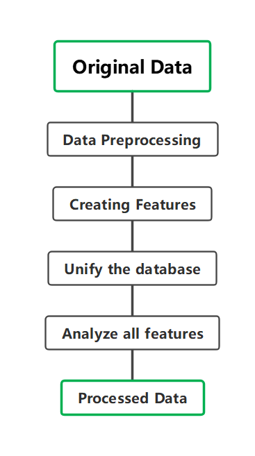
Figure 1. Processing of data.

2.2. Proposed approach

A model with the best recall is required since the objective of this project is to forecast each match as precisely as possible based on the information and data already available. A library called scikit-learn is being used to train these two models. After training, these two models are being tested: the GB and the RF model. After the pre-preprocessing of the data, these data and features are used to train these two models and use Receiver Operating Characteristic (ROC) graphs and confusion matrixes to evaluate the performance of these models. ROC graphs are handy when finding whether the model is overfit or underfit, and the confusion matrix is being used to calculate the recall rate and accuracy of the model. Figure 2. Shows this process.

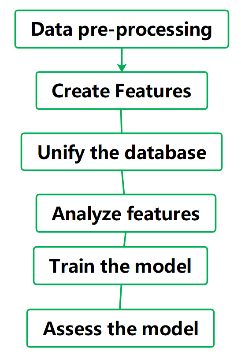
Figure 1. The overall process of the project.

2.2.1. Random Forest Model. A popular algorithm in ML for performing both classification and regression tasks is the RF model. It uses an integrated strategy that makes use of several little estimators, such as decision trees, to provide unique predictions. For regression tasks, the RF model’s output is either the mean or average prediction of each tree or for classification tasks, the class that the majority of trees choose. The RF Model’s ability to process a large number of input variables without deleting any of them is one of its key advantages. It is a great method for feature selection because it can evaluate how important each feature is in a classification problem. Additionally, even when a sizable portion of the data is missing, it can still maintain accuracy thanks to an efficient estimation method. A random selection of characteristics and data points is used to establish each decision tree in the RF Model. The selection procedure’s randomness lowers the possibility of overfitting and increases the model’s precision. The model also lends itself to large-scale data analysis and is simple to parallelize. In conclusion, the RF Model is a reliable and flexible algorithm that may be used for a number of different functions, including prediction, classification, and feature selection. Its ability to handle large datasets, estimate missing data, and maintain accuracy makes it a popular choice among data scientists and researchers.

2.2.2. GB model. The GB Model, a method that applies machine learning to classification and regression problems, generates a prediction model in the form of a collection of weak prediction models. By allowing the optimization to use any differentiable loss function, it gradually builds a model and generalizes it. Through a process of iteration, it turns multiple weak “learners” into one powerful one. The most straightforward explanation is to “guide” the value of the model’s predictive form by the diminution of the mean square error, and in the least squares regression, accomplishing the correct guidance by lowering the value of the mean square error is the goal. The GB approach creates progressively less accurate prediction models, while they may also be built more quickly. Each model seeks to anticipate the error made by the one before it. A weak learning model outperforms random predictions by a small margin. The algorithm is based on the idea that a predictor can be improved by combining many weak learners (like shallow trees). The succeeding models make an effort to identify and forecast the error that the preceding model left behind.

2.2.3. Model evaluation and visualization. The performance of an ML model on a set of test data is summarised in the confusion matrix, which can be seen in Table 1. The efficacy of classifying models, whose objective is to predict a category label for every input’s occurrence, is typically measured using this metric.

Table 1. The example of a confusion matrix. TP stands for the number of positive instances that are correctly classifier while FP is the number of negative instances. Meanwhile, FN and TN are the numbers of positive and negative instances.

By dividing the quantity of TPs and FNs by the number of TPs, the recall rate can be computed. The sensitivity or true positive rate are other names for it. It measures the percentage of real positive cases that the model correctly identified, making it a helpful statistic to evaluate a prediction model’s efficacy. The way the model is able to recognise affirmative situations is evidenced by its significant recall rate. The formula for the recall rate is written as:

\( Recall Rate= \frac{TP}{(TP+FN)} \) (1)

Because it indicates the percentage of accurate predictions, accuracy is a helpful indicator for assessing a prediction model’s performance. The formula for accuracy is written as:

\( Accuracy= \frac{(TP+TN)}{(TP+TN+FP+FN)} \) (2)

In binary classification problems, the ability of a model to correctly identify positive instances is measured using a performance metric called precision. The ratio of properly anticipated positive outcomes to all positive outcomes, which includes both correctly and wrongly predicted positive outcomes, is how this term is defined. To put it differently, precision gauges the percentage of accurate predictions that are classified as true positives. The formula of precision will be written as:

\( Precision= \frac{TP}{TP+FP} \) (3)

2.3. Implemented details

The program uses Python 3.9.16 and the scikit-learn library to achieve both the RF and GB model. The data is visualized by using the Seaborn and Matplotlib libraries. The program is carried out on a 64-bit Windows PC with an Intel Core i5-11400H processor and an NVIDIA GeForce RTX 3050Ti Laptop graphics card. Both these two methods are being used to simulate the results of each match in a series of games. For GB, the value used for performing grid tests is [0.01, 0.1, 0.5]. By establishing an upper limit for the bare minimum amount of samples in a leaf, which are [3, 5], defining a value of the lowest number of samples necessary to be at a leaf node aids in controlling overfitting. The maximum depth of a single tree was [3, 5, 10] and the number of estimators was set to be [100, 200]. In addition, this paper sets the maximum depth to 20, the minimum samples split to 10 and the maximum number of leaf nodes to 175 for RF. At a leaf node, a minimum of five samples is necessary.

3. Result and discussion

After data preprocessing, creating and assessing features, the next step is to train the models. Based on the program-generated tables, a detailed comparison of the GB and RF Models is made in this section. The evaluation uses two different types of graphs. The ROC curve is a graph that displays the true positive rate (TPR) against the false positive rate (FPR) at different threshold settings, illustrating the performance of a binary classifier system. The area under the ROC curve (AUC) is a measure of the classifier’s performance, with the 2D area extending from the origin (0, 0) to (1.0, 1.0). It gives a total performance evaluation across all potential classification thresholds. The AUC ranges from 0 to 1, with 1 denoting the best possible classifier and 0.5 denoting a classifier that performs no better than random chance. A classification model’s performance is described using a confusion matrix. It shows TP, FP, TN, and FN predictions. By performing a few straightforward computations, it is possible to evaluate the model’s performance based on its recall rate, precision and other metrics.

The ROC curve for the RF model is shown in Figure 3. The AUC score on the test set is 0.79, and on the training set, it is 0.96, as indicated by the graph’s title. According to the data provided about the training set (blue line) and test set (orange line) in the graph, it is obvious that the training dataset’s AUC result is greater than the test dataset’s, suggesting that the predictive model may be a little bit overfitted, which means that it has learned to perform well on the training data but does not generalize as well to new data.

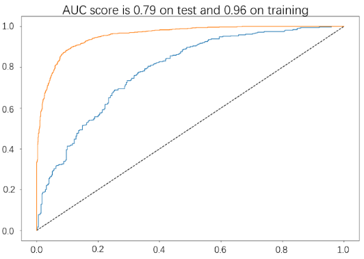
Figure 2. ROC curve of the RF model.

Figure 4. is the confusion matrix of the RF model. In the graph, the four quadrants represent the four possible outcomes of a binary classification problem. The orange quadrant represents TP, which is 242 in this case. The purple quadrant represents FP, which is 108. The black quadrant and the beige quadrant represent FN and TN, the value is 101 and 288 respectively. From this information, it is easy to calculate various performance metrics for the RF model. The accuracy and other two important metrics of the model are shown in Table 2. The value of accuracy indicates that the model correctly classifies about 71.72% of the instances. The precision means that about 69.14% of the instances predicted by the model as positive are positive. Recall, also known as sensitivity, illustrates that the model correctly identifies about 70.55% of positive instances.

Table 2. Measurement parameters of the RF model.

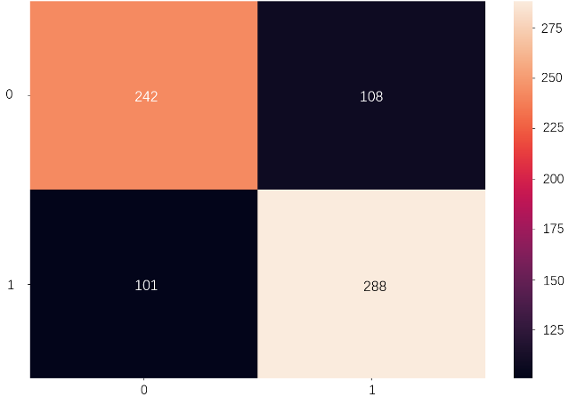
Figure 3. Confusion matrix of the RF model.

The same analysis process is being carried out on the GB model as well. Based on Figure 5, it can be inferred that the AUC score is 0.80 for both the test set and training set. This shows that the GB model does not seem to have an overfitting problem.

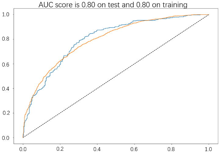
Figure 4. ROC Curve of GB model.

Figure 6. is the confusion matrix of the GB model. The meaning of each quadrant is as same as before, but the numbers and values are different. The orange quadrant represents the number of true positives (TP), which is 245 in this case. The purple quadrant represents the number of false positives (FP), which is 105. The black quadrant and the beige quadrant represent false negatives (FN) and true negatives (TN), the value is 87 and 302 respectively. From this information, it is possible to calculate the value of the accuracy, recall rate and precision. The accuracy and other two important metrics of the model are shown in Table 3.

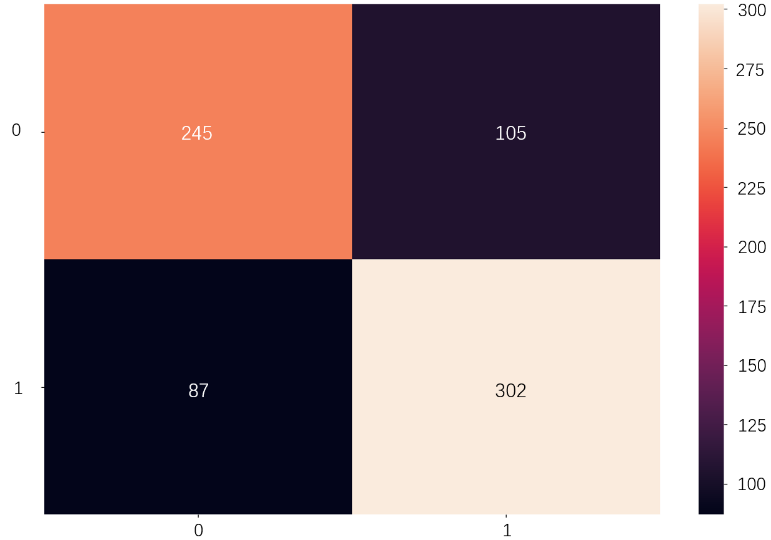
Figure 5. Confusion matrix of GB model.

Table 3. Measurement parameters of the GB model.

Same as before, the accuracy shows that the model correctly classifies about 74.02% of the instances. The precision means that about 70.00% of the instances predicted by the model as positive are positive. The recall rate illustrates that the model correctly identifies about 73.80% of positive instances. Table 4. summarizes all the data obtained from the four figures above. This table helps evaluate the performance difference between the two models.

Table 4. Summary of measurement parameters of two models.

From Table 4, it is easy to find out that both the RF and GB models have similar AUC scores on the test set, with the RF model scoring 0.79, while the GB model received a slightly better score of 0.80. However, the AUC score on the training set is much higher for the RF model (0.96) than for the GB model (0.80). This suggests that the RF model may be overfitting to the training data, meaning that it has learned to perform very well on the training data but does not generalize as well to new data. In terms of other performance metrics, the GB model has a higher accuracy (0.7402), precision (0.7000) and recall (0.7380) compared to the RF model, which has an accuracy of 0.7172, a recall of 0.7055 and a precision of 0.6914. In general, when choosing between two models with similar performance on the test set, it is a good idea to choose the simpler model or the model that is less prone to overfitting. Since the GB model has a lower AUC score on the training set than the RF model and is thought to be less prone to overfitting, it appears that it might be a better option in this situation. In addition, in terms of precision, accuracy and the value of the recall rate, the GB model performs better than the RF model. Figure 7. shows the course of play and the result of a complete World Cup match predicted by this program based on the latest available dataset.

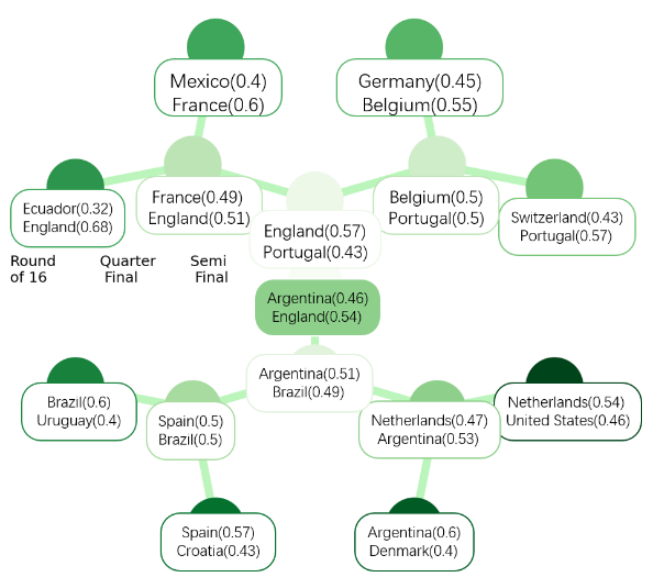
Figure 6. The predicted result of the World Cup.

4. Conclusion

This study introduces ML techniques to forecast the FIFA World Cup results, specifically RF models and GB models. It is possible to assess the effectiveness of the two models and choose the most appropriate one by using feature engineering techniques to produce a suitable dataset for ML. The capability of the RF model was evaluated and it was determined that it did not perform as well as the GB. The accuracy, precision, and recall of the GB model were all higher while the AUC score on the training set was lower. According to these findings, the GB model is the most effective option for forecasting the FIFA World Cup results. In the future, this study plans to expand the research by considering additional factors that may influence the outcome of a match. Factors such as player ratings, and degrees of aggression when attacking or team-defending ratings will be added to the model in the next stage of the research.

References

[1]. 2022 financial highlights FIFA Publications FIFA Publications. https://publications.fifa.com/en/annual-report-2022/finances/2019-2022-cycle-in-review/2022-financial-highlights/
[2]. Shobana G Suguna M 2021 Sports prediction based on RF algorithm In Springer Proceedings in Materials pp 993–1000
[3]. R Hucaljuk J Rakipović A 2011 Predicting football scores using machine learning techniques//2011 Proceedings of the 34th International Convention MIPRO IEEE pp 1623-1627
[4]. Boi Ross W J Orr M 2022 Predicting climate impacts to the Olympic Games and FIFA Men’s World Cups from 2022 to 2032 Sport in Society 25(4): pp 867-888
[5]. Groll A 2018 Prediction of the FIFA World Cup 2018 - A RF approach with an emphasis on estimated team ability parameters arXiv.org 1806.03208
[6]. Pinasthika S J Fudholi D R 2022 World Cup 2022 Knockout Stage Prediction Using Poisson Distribution Model IJCCS (Indonesian Journal of Computing and Cybernetics Systems) 17(2)
[7]. Yoon J 2020 Forecasting of real GDP growth using machine learning models: GB and RF approach Computational Economics 57(1): pp 247–265
[8]. Glen S 2019 Decision Tree vs RF vs GB Machines: Explained Simply Data Science Central
[9]. International football results 2023 Kaggle. https://www.kaggle.com/datasets/martj42/international-football-results-from-1872-to-2017
[10]. FIFA World Ranking 2023 Kaggle. https://www.kaggle.com/datasets/cashncarry/fifaworldranking
Cite this article
Meng,X. (2024). Soccer match outcome prediction with random forest and gradient boosting models. Applied and Computational Engineering,40,99-107.
Data availability
The datasets used and/or analyzed during the current study will be available from the authors upon reasonable request.
Disclaimer/Publisher's Note
The statements, opinions and data contained in all publications are solely those of the individual author(s) and contributor(s) and not of EWA Publishing and/or the editor(s). EWA Publishing and/or the editor(s) disclaim responsibility for any injury to people or property resulting from any ideas, methods, instructions or products referred to in the content.
About volume
Volume title: Proceedings of the 2023 International Conference on Machine Learning and Automation
© 2024 by the author(s). Licensee EWA Publishing, Oxford, UK. This article is an open access article distributed under the terms and
conditions of the Creative Commons Attribution (CC BY) license. Authors who
publish this series agree to the following terms:
1. Authors retain copyright and grant the series right of first publication with the work simultaneously licensed under a Creative Commons
Attribution License that allows others to share the work with an acknowledgment of the work's authorship and initial publication in this
series.
2. Authors are able to enter into separate, additional contractual arrangements for the non-exclusive distribution of the series's published
version of the work (e.g., post it to an institutional repository or publish it in a book), with an acknowledgment of its initial
publication in this series.
3. Authors are permitted and encouraged to post their work online (e.g., in institutional repositories or on their website) prior to and
during the submission process, as it can lead to productive exchanges, as well as earlier and greater citation of published work (See
Open access policy for details).