1. Introduction

In today’s digital age, recommendation systems have emerged as powerful tools that subtly influence daily lives. They have been under development since the early 1990s [1]. These sophisticated algorithms are the linchpin of the digital world, seamlessly connecting us to content, products, and experiences tailored to the unique tastes and preferences. At the heart of recommendation systems lies a complex web of algorithms meticulously designed to predict user preferences and curate suggestions accordingly. These systems thrive on data – vast oceans of it – analyzing user behaviors, historical interactions, and item attributes to uncover intricate patterns and correlations [2]. Armed with these insights, recommendation systems craft personalized recommendations that engage and captivate users. The versatility of recommendation systems knows no bounds, permeating numerous facets of the daily lives: Recommendation algorithms have completely changed how consumers shop online in the world of e-commerce. Online retail giants like Amazon rely on these systems to navigate customers through a seemingly endless array of products [3]. By meticulously analyzing purchase histories and customer profiles, these systems suggest items that align seamlessly with users’ preferences and past buying habits. Platforms like Netflix and Spotify have made content discovery an art form in the world of streaming services. [4,5]. These systems meticulously examine users’ past viewing or listening behaviors, ensuring that the next movie or music selection feels tailor-made for each individual. In the sphere of news and content, recommendation systems silently curate the daily news feed. They sift through a vast sea of articles and videos, delivering content that mirrors the interests and aligns with the reading habits.

One of the key technologies is the collaborative filtering (CF)-based recommendation system. [6,7]. CF presents a systematic approach which furnishes users with tailored recommendations. Within CF, Singular Value Decomposition (SVD) and Alternating Least Squares (ALS) emerge as significant algorithms. This paper mainly compares SVD and ALS two algorithms based on matrix decomposition, explains the principle of the two algorithms in detail and analyses the differences in accuracy caused by their subtle differences. Through this exploration, the paper aims to equip researchers, practitioners, and stakeholders with the knowledge needed to navigate the ever-evolving landscape of recommendation systems effectively.

2. Method

2.1. Dataset

The dataset under consideration in this research comes from a curation project led by Dr. Jianmo Ni at UCSD. This dataset consists of links, product metadata, and reviews. Since the algorithms involved in this paper are all based on matrix decomposition, the reviewer ID, product ID and rating are mainly used.

2.2. Dataset Preprocessing

The role of data preprocessing is to conduct a comprehensive exploration of data attributes, including data complexity, component elements, distribution characteristics, etc. This comprehensive analysis provides an accurate basis for the establishment of the recommendation system, and also provides an essential reference for the selection and discussion of the algorithm. Therefore, before starting the subsequent algorithm, the necessary data preprocessor is essential, and Table 1 and Table 2 demonstrates the data statistics and the statistics of df1 in the dataset respectively.

Table 1. Dataset Statistics.

Since the data is very big. Consider electronics_df1 named data frame with first 50000 rows and all columns from 0 of dataset:

Table 2. Dataset Statistics of electronics_df1.

In Electronic_df1, there is no missing value. Therefore, the dataset does not need to do much additional preprocessing. These foundational metrics, coupled with descriptive statistics such as mean, standard, minimum, and maximum ratings, collectively afford a comprehensive contextualization of the dataset characteristics across various dimensions. It can be seen from the data that ratings mean as high as 4.07. The distribution diagram of ratings is displayed in Figure 1 to help with comprehension of the data set’s intuitive distribution.

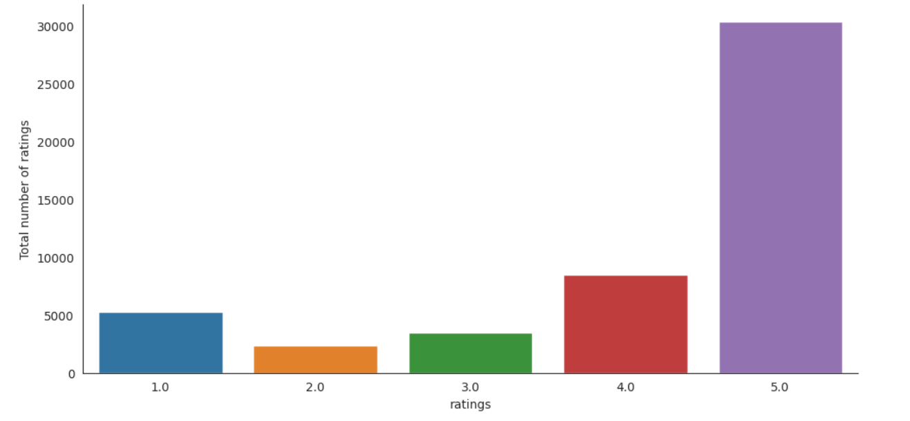
Figure 1. Histogram on Ratings for Electronics_df1 (Figure credit: Original).

According to the histogram, it can be found that the evaluation of full marks accounts for more than half, the evaluation of four points is about one-fifth, and the evaluation of one point is slightly less than four points, but it also reaches one-tenth of the total number of ratings, indicating that users rarely give neutral ratings when evaluating, and usually three kinds of evaluations are very satisfied, basically satisfied and very dissatisfied.

2.3. Models

The performance of the underlying dataset is assessed using Singular Value Decomposition and Alternating Least Squares.

2.3.1. Singular Value Decomposition (SVD)

SVD, a technique originating from the generalization of eigen decomposition principles for square normal matrices to matrices of arbitrary dimensions, made a significant impact when introduced by Simon Funk during the era of the Netflix Prize competition [8].

SVD achieves a decomposition that can be applied to rectangular matrices of real numbers by utilizing the eigen-decomposition of a positive semi-definite matrix. The core concept involves breaking down any matrix into three fundamental components: one diagonal matrix and two orthonormal matrices. When employed with a positive semi-definite matrix, SVD is essentially equivalent to eigen-decomposition. if A is a rectangular matrix, its SVD decomposes it as:

\( A=PΔ{Q^{T}} \) (1)

Here, \( P \) is the matrix \( {AA^{T}} \) ‘s (normalized) eigenvectors. The left singular vectors of \( A \) are referred to as the columns of \( P \) . The columns of \( Q \) are known as the right singular vectors of \( A \) , and \( Q \) is a reference to the (normalized) eigenvectors of the matrix \( {A^{T}}A \) . \( Δ \) is the diagonal matrix of the singular values. In recommendation system, A is considered as the original user-item matrix, \( P \) is the user matrix, \( Δ \) can be considered as the weight between users and items, and \( {Q^{T}} \) is the transpose of the item matrix. The singular value matrix \( Δ \) represents important features in the data. By retaining only the first few singular values in the \( Δ \) matrix, it could receive a low-dimensional approximate matrix, reducing the dimensionality of the original data. This helps filter out noise and unimportant information while retaining the main features of the data. As a result, it can be observed that SVD is not suitable for excessively sparse data and encounters the cold start problem. When additional users or objects are added to the system, SVD necessitates a complete model recalculation, rendering it incapable of offering meaningful recommendations immediately.

In summary, SVD possesses certain advantages within recommendation systems, particularly in the realms of personalized recommendations and dimensionality reduction. However, it also exhibits constraints, notably when dealing with sparse data and real-time recommendations. In practical applications, it is often necessary to contemplate alternative recommendation algorithms and technologies to compensate for the limitations of SVD.

2.3.2. Alternating Least Squares (ALS)

ALS algorithm is fundamentally item-based collaborative, and in recent years, model-based recommendation algorithms like ALS have been successfully applied at Netflix, resulting in significant improvements in performance [9]. ALS utilizes machine learning algorithms to establish interaction models between users and items, enabling predictions of new items.

The core idea of ALS is to connect user interests with items through latent factors, based on user behavior to discover latent themes and categories. Then, it automatically clusters item and assigns them to different categories/themes (representing user interests). The m×k user matrix U and the k×n item matrix M are the two components that matrix factorization algorithms utilize to deconstruct the m×n co-occurrence matrix R. There, k is the dimension of the latent vectors, n is the number of items, and m is the number of users. The size of k influences the strength of the latent vector’s expressive capability, with larger k values conveying more information.

A k-dimensional latent vector represents each user and object. Therefore, to calculate a user’s rating or other implicit behavior for a specific item, only the inner product of the corresponding vectors is needed to compute.

\( {p_{ij}}=U_{i}^{T}{M_{J}}= \lt {u_{i}},{m_{j}} \gt \) (2)

Here, \( p \) reference to the corresponding vectors. \( U \) = [ \( {u_{i}} \) ] is the user feature matrix, where \( {u_{i}} \) denotes the i-th column of \( U \) and \( M \) =[ \( {m_{j}} \) ] is the item feature matrix, where \( {m_{j}} \) means the j-th column of \( M \) .

For users and items with interaction behavior, their rating bias is represented as r-p. When considering an individual sample:

\( L(r,u,m)={(r-p)^{2}}={(r- \lt u,m \gt )^{2}} \) (3)

Here, r represents the rating score of this individual sample. Therefore, the loss function on the entire sample is:

\( L(R,U,M)={sum_{(i,j)∈I}}​L({r_{ij}}​,{u​_{i}},{m_{j}}​) \) (4)

where \( I \) is the index set of the known ratings. To minimize this loss function, the objective function is formulated as follows:

\( L_{λ}^{reg}​(R,U,M)=\sum _{(i,j)∈I}[{({r_{ij}}​-{u_{i}}​m_{j}^{T})^{2}}+λ({∣∣{u_{i}}​∣∣^{2}}+{∣∣{m_{j}}​∣∣^{2}})]​ \) (5)

In the formula, L2 regularization is employed to penalize the model’s parameters to mitigate overfitting issues.

2.4. Evaluation Methods

RMSE: RMSE (Root Mean Square Error) is a commonly used metric for evaluating model performance, especially in regression problems [10]. It is used to quantify the size of the discrepancy or error between the values that a model predicts and the actual values that are observed.

\( RMSE=\sqrt[]{\frac{1}{m}\sum _{i=1}^{m}{(h({x_{i}})-{y_{i}})^{2}}} \) (6)

Here, The i-th data point’s actual observed value is denoted by \( h({x_{i}}) \) , while the i-th data point’s forecasted value is denoted by \( {y_{i}} \) . \( m \) refers to the whole amount of data points.

Fundamentally, RMSE measures the average size of prediction mistakes. As smaller prediction errors are represented by lower RMSE values, better predictive ability is indicated.

3. Result

SVD and ALS have been applied separately to the previous dataset, and the following will show the top four recommended items for the first three users by each algorithm, as demonstrated in Table 3 and 4 respectively.

Table 3. Recommended items for users from SVD.

Each table provides personalized recommendations for an individual user, with the “user_predictions” column indicating the predicted preferences or ratings for each recommended item. Higher values indicate stronger recommendations based on the algorithm’s predictions. Some items (e.g., “B00001O2YP”) appear in the recommendations for multiple users, suggesting that these items may enjoy wider popularity or be better suited for a broader audience.

Table 4. Recommended items for users from ALS.

Similar to SVD, these ALS recommendations are personalized for each user, offering items tailored to their potential preferences. Unlike SVD, there are no common items recommended across different users.

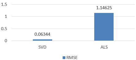
Figure 2. RMSE comparison between ALS, SVD (Figure credit: Original).

The results of this comparative evaluation reveal that the SVD model attains the lower RMSE values than the ALS model, which the RMSE of SVD equals to 0.06344 and the ALS equals to 1.14625, as displayed in Figure 2.

4. Discussion

In this paper, RMSE was used to evaluate the two models respectively, and the results showed that SVD model performed significantly better than ALS, which may be caused by the following four reasons: a smaller subset is chosen, For small-scale datasets, SVD often finds better low-dimensional representations with lower computational costs because it directly decomposes the entire rating matrix. ALS may require more iterations to converge, especially on large-scale datasets. At the same time, this will also cause the data to be less sparse, ALS is typically better suited for handling sparse data because it can effectively deal with missing data points. ALS updates the latent feature vectors for users and items alternately, allowing modeling in the presence of a large number of missing values. In data processing, user data with more than five ratings is selected as a subset, which may lead to a certain linear relationship in the subset, that is, users give higher ratings to items with higher ratings. And SVD can better capture such relationships. ALS, on the other hand, minimizes the loss function through iterative steps and can also be used to discover linear relationships, but its advantage typically lies in adapting to non-linear relationships. This may also have created specific data noise, SVD relatively robust to noise or outliers in the data. Outliers do not usually have a significant impact on singular value decomposition. In contrast, ALS updates the model based on user-item interactions in each iteration and may be more sensitive to noise.

5. Conclusion

In this comprehensive analysis and evaluation of recommender models, this work delves into the performance of two prominent matrix decomposition techniques, specifically SVD and ALS, within the context of the Amazon dataset. Through meticulous evaluation, this work aims to unravel the nuanced intricacies of these models, shedding light on their performance characteristics, predictive prowess, and a thorough exploration of the factors that might influence their precision and relevance.

Upon subjecting these models to rigorous scrutiny, the evaluation results unveil noteworthy disparities. SVD emerges as the frontrunner, demonstrating a notably superior performance on this dataset as evidenced by a remarkably low Root Mean Square Error (RMSE) of merely 0.06344, in stark contrast to ALS’s RMSE of 1.14625. These findings underline the importance of selecting an appropriate recommendation algorithm that aligns with the dataset’s underlying patterns and characteristics.

Furthermore, this analysis delves into the pervasive issue of data sparsity, which looms large as one of the principal challenges confronting recommendation systems. The paper not only highlights the existence of this challenge but also underscores the pressing need for ongoing research and continuous improvements to tackle it effectively. The complexities inherent in handling sparse data underscore the evolving nature of recommendation system research, opening doors to innovative solutions and strategies for enhancing their accuracy and relevance. As the field advances, addressing data sparsity remains a pivotal area for exploration and innovation.

References

[1]. Resnick, P., & Varian, H. R. (1997). Recommender systems. Communications of the ACM, 40(3), 56-58.
[2]. Beheshti, A., Yakhchi, S., Mousaeirad, S., Ghafari, S. M., Goluguri, S. R., & Edrisi, M. A. (2020). Towards cognitive recommender systems. Algorithms, 13(8), 176.
[3]. Linden, G., Smith, B., & York, J. (2003). Amazon. com recommendations: Item-to-item collaborative filtering. IEEE Internet computing, 7(1), 76-80.
[4]. Bennett, J., & Lanning, S. (2007). The netflix prize. In Proceedings of KDD cup and workshop, 2007, 35.
[5]. Madathil, M. (2017). Music recommendation system spotify-collaborative filtering. Reports in Computer Music. Aachen University, Germany 1-4.
[6]. Su, X., & Khoshgoftaar, T. M. (2009). A survey of collaborative filtering techniques. Advances in artificial intelligence, 1-19.
[7]. Koren, Y., Rendle, S., & Bell, R. (2021). Advances in collaborative filtering. Recommender systems handbook, 91-142.
[8]. Kalman, D. (1996). A singularly valuable decomposition: the SVD of a matrix. The college mathematics journal, 27(1), 2-23.
[9]. Zhou, Y., Wilkinson, D., Schreiber, R., & Pan, R. (2008). Large-scale parallel collaborative filtering for the netflix prize. In Algorithmic Aspects in Information and Management: 4th International Conference, 4, 337-348.
[10]. Herlocker, J. L., Konstan, J. A., Terveen, L. G., & Riedl, J. T. (2004). Evaluating collaborative filtering recommender systems. ACM Transactions on Information Systems, 22(1), 5-53.
Cite this article
Zhao,T. (2024). Performance comparison and analysis of SVD and ALS in recommendation system. Applied and Computational Engineering,49,142-148.
Data availability
The datasets used and/or analyzed during the current study will be available from the authors upon reasonable request.
Disclaimer/Publisher's Note
The statements, opinions and data contained in all publications are solely those of the individual author(s) and contributor(s) and not of EWA Publishing and/or the editor(s). EWA Publishing and/or the editor(s) disclaim responsibility for any injury to people or property resulting from any ideas, methods, instructions or products referred to in the content.
About volume
Volume title: Proceedings of the 4th International Conference on Signal Processing and Machine Learning
© 2024 by the author(s). Licensee EWA Publishing, Oxford, UK. This article is an open access article distributed under the terms and
conditions of the Creative Commons Attribution (CC BY) license. Authors who
publish this series agree to the following terms:
1. Authors retain copyright and grant the series right of first publication with the work simultaneously licensed under a Creative Commons
Attribution License that allows others to share the work with an acknowledgment of the work's authorship and initial publication in this
series.
2. Authors are able to enter into separate, additional contractual arrangements for the non-exclusive distribution of the series's published
version of the work (e.g., post it to an institutional repository or publish it in a book), with an acknowledgment of its initial
publication in this series.
3. Authors are permitted and encouraged to post their work online (e.g., in institutional repositories or on their website) prior to and
during the submission process, as it can lead to productive exchanges, as well as earlier and greater citation of published work (See
Open access policy for details).