1. Introduction

Based on the dramatic development and popularization of the Internet of Things, the retail industry with physical stores is taking the challenge of the unprecedented influence on the environment [1]. Specifically, consumers' shopping habits and preferences are fundamentally changing in the digital era. This indicates that traditional supermarkets and grocery retailers have had to continually adapt their business strategies to this new market environment [2].

This study focuses on data from customers placing orders using grocery delivery data in Tamil Nadu, India [3]. It aims to provide retailers with valuable insights through in-depth consumer behavior analysis and related sales data. This dataset provides an opportunity to engage in exploratory data analytics and data visualization, and by revealing patterns, trends, correlations, and efficiency of different regression models, retailers can be recommended to optimize their marketing, pricing, and product strategies to increase sales and revenue and reduce the opportunity cost.

As machine learning technology continues to evolve, its use in the retail industry has become increasingly common [4,5]. Using machine learning algorithms, this work can build sales forecasting models to predict future sales trends by analyzing historical data, thus helping retailers make more accurate decisions in inventory management and supply chain optimization.

The importance of this study lies not only in providing insights into consumer behavior and market trends but also in providing retailers with a framework for data-driven decision-making. By analyzing a large amount of order data and customer behavior, this work can discover the patterns hidden behind the data and provide a scientific basis for retailers' business strategies. Implementing this study is expected to provide valuable insights to retail industry practitioners, helping them maintain a competitive edge in this highly competitive market. At the same time, this study is also expected to provide a compelling reference framework for future research in related fields. These efforts contribute in a small way to the future development of the retail industry.

2. Method

2.1. Dataset

The dataset contains order ID, customer name, category, subcategory, address, order date, region, sales, and discount. There are different types of forecasts. Specifically, Sales Forecasting Models Using historical sales data, product categories, discounts, and other features, a sales forecasting model can be built to predict sales in a future period to help retailers make reasonable inventory and supply chain management decisions [3].

There is also a data model that can improve user satisfaction. Machine learning algorithms can analyze and classify customers to identify high-value customers and provide personalized services and recommendations based on a customer's historical purchasing behavior and consumption amount.

Product recommendation systems are standard models today, but most are used for online shopping, such as Amazon. Online supermarket purchases have yet to be entirely popularized. Based on the user's purchase history and product categories, subcategories, and other information, a personalized product recommendation system can be constructed to provide users with customized shopping advice and improve the transaction conversion rate.

Due to the unstable supply chain in recent years, the cycle arrangement of incoming goods has become a relatively tricky point for retailers to judge. That's why some models choose to measure customer churn predictions. Using a customer's order history data, purchase frequency, and other characteristics, a customer churn prediction model can help retailers identify potential churn customers promptly and take steps to retain them.

Similarly to solidify inventory and stocking in the supply chain, the data is based on the collection of temporal characteristics, which can be used to build a model to predict sales at different times of the year (e.g., holidays, weekends, etc.) to make timely adjustments to marketing campaigns.

This dataset also contains geographic sales forecasts. Orders come from selected branches in India. The retailer's head office can be based on characteristics such as region, season, product category, etc. It can build a model to predict sales in different regions in a certain period in the future to rationalize inventory and resources. This reduces the problem of loss of goods and failure to fulfill sales performance.

The selling price category models can be analyzed in two ways through data. One type is the discount optimization strategy. By analyzing the impact of different discount levels on sales, a model can be built to optimize the discount strategy to maximize sales and profits. The other is based on product categories, sales data, and cost information. A pricing optimization model can be built to ensure that product pricing meets market demand and profit maximization goals. These models can be projected and simulated with the dataset taken for this research.

2.2. Data Cleaning

After obtaining the supermarket sales dataset, which includes variables such as order ID, customer name, product category, subcategory, order address, order date, area sales, and discount information. In the data preprocessing phase, the following operations were performed:

Dealing with Missing Values: Check whether there are any missing values in the dataset, and if so, process them accordingly, either by deleting or filling in the missing values.

Data transformation and coding: coding the category-based variables for subsequent modeling and analysis. For example, the region is coded in the dataset as Southeast, Northwest, and Central by converting it to a number for replacement.

2.3. Models

2.3.1. Linear Regression. When using characteristics as independent variables to see a linear relationship between them and sales, select specific characteristics and build a linear regression model with them as independent variables and sales as the dependent variable [6]. Based on the data, the following linear regression model could be constructed.

\( Profit = {β_{0}} + {β_{1}}×Discount + {β_{2}}×Region+{β_{3}}×Sales+ϵ \) (1)

where \( β \) and \( ϵ \) denote model parameters.

2.3.2. Polynomial Regression. In this study, polynomial regression models were considered to fit possible nonlinear relationships better than linear regression models. Polynomial regression can deal with complex relationships that linear models do not explain well by introducing higher-order features. Introducing higher-order powers allows more flexibility in fitting nonlinear relationships in the data. In many real-world circumstances, the relationship between the independent and dependent variables is frequently not a simple linear relationship and may contain curves, surfaces, or more complex forms. Introducing higher-order specials improves the adaptability and predictive power of the model [7]. Example with degrees equals two:

\( Profit ={β_{0}}+{β_{1}}×Discount×{β_{2}}×Discoun{t^{2}}+{β_{3}}×Region+{β_{4}}×Regio{n^{2}}+{β_{5}}×Sales+{β_{5}}×Sale{s^{2}}+ϵ \) (2)

where \( β \) and \( ϵ \) denote model parameters.

2.3.3. Ridge Regression. Ridge regression is also used to forecast and analyze profits. Ridge regression provides an effective way to improve the performance of linear regression models. Introducing a regularization term, also known as a ridge penalty, limits the size of the model parameters and effectively controls the complexity of the model [8]. This feature makes ridge regression particularly useful when dealing with features that exhibit multicollinearity or when the number of features exceeds the number of samples. Ridge regression prevents overfitting on the training set and improves the model's generalization ability, resulting in better performance on unseen data. When using ridge regression, careful selection of the regularization parameter (alpha) is critical to obtain optimal model performance. Often, methods such as cross-validation are used to select appropriate alpha values. In conclusion, ridge regression is a powerful and versatile tool to improve the performance and stability of linear regression models in various practical applications. The following equation gives a common practical ridge estimator:

\( {\hat{β}_{R}}=({X^{T}}X+λI{)^{-1}}{X^{T}}y \) (3)

Typically, ridge regression makes a trade-off between prediction bias and variance. The regression will call for a relatively small bias and, thus, a significant reduction in the mean square error.

\( MSE=E(\hat{β}-β{)^{2}}=(E(\hat{β}-β){)^{2}}+(E(\hat{β}-E\hat{β}){)^{2}}={bias^{2}}+variance \) (4)

2.3.4. Logistic Regression. Logistic regression is a classical statistical learning method widely used to solve binary classification problems. Logistic regression is a method used to solve classification problems that output a probability value between 0 and 1, indicating the likelihood of an event occurring. In this essay, the exploration of Logistic Regression is based on the application scenarios provided by the data [9]. The core components of the Logistic Regression model include the Sigmoid function, the Hypothesis function, and the Loss function. By minimizing the logarithmic loss function, such models can find the optimal model parameters using optimization algorithms such as gradient descent. Logistic regression is valuable as a simple but effective classifier in many practical applications.

Logistic regression has some limitations. For instance, logistic regression will perform relatively poorly when market analysis involves nonlinear relationships. It cannot directly handle complex nonlinear data and may require additional feature engineering or consideration of more complex models. The original logistic regression is used for binary classification problems, which require additional processing for multi-category classification problems, such as one-to-many or many-to-many strategies [10]. The multiple binary logistic regression model is the following:

\( π(X)=\frac{exp⁡({β_{0}}+{β_{1}}{X_{1}}+…+{β_{k}}{X_{k}})}{1+exp⁡({β_{0}}+{β_{1}}{X_{1}}+…+{β_{k}}{X_{k}})}=\frac{exp⁡(Xβ)}{1+exp⁡(Xβ)}=\frac{1}{1+exp⁡(-Xβ)} \) (5)

2.4. Evaluation Standards

The regression results of this code experiment were judged using Mean Square Error (MSE) and R-squared (R²). MSE is a metric used to assess the predictive accuracy of a model. Smaller values indicate that the model's predicted values are less different from the actual values, so the model performs better. R² takes values from 0 to 1. R² equals one, which means that the model fits the data perfectly. The model explains all the variance in the target variable, and the predicted values are the same as the actual values. R² equals zero, which indicates that the model's predicted values are essentially the same as the mean of the target variable. R² less than zero means the model's predictions are worse than if the mean had been used directly.

3. Results

3.1. Result of Variance Inflation Factor (VIF) and Quantile-Quantile (Q-Q) Plot

The selected variables predict supply chain sales, discounts, and purchases and analyze whether profits correlate with regions. For this experiment, the predictor (Y) is profit, and the response variable (X) is discount, sales, and region. Before the start of the experiment, the available data were used to make speculations and outlooks on the experiment's results. The quantile-quantile plot and VIF data can approximate the relationship between the variables and verify the future choice of the regression algorithm.

VIF measures whether the current data are strongly correlated and suitable for multiple regression modeling. Results are shown in Table 1. Specifically for the predictor variables "Sales," "Discounts," and "Region," the VIF values are close to 1 to show that the correlation between these variables is not strong. According to the definition of VIF, a VIF value around one usually indicates almost no multicollinearity. Because this means that each predictor ("Sales," "Discount," and "Region") can provide unique information for the prediction of the dependent variable, it is crucial to analyze the general situation of the data before proceeding with the model selection. Suppose the independent variables chosen for the experiment appear highly correlated. In that case, this can lead to problems in the regression analysis, as isolating the individual effects of the correlated variables on the dependent variable is challenging. Overall, this speculative step also avoids understanding the genuine relationship between each independent and dependent variable, which may become difficult.

Table 1. Result of VIF factors.

In statistical analysis, Q-Q plots are a valuable diagnostic tool for checking the assumptions behind many statistical tests and models. It allows for a visual assessment of whether the data in an experiment conforms to the hypothesized distribution, which is essential for making valid inferences due to the singularity and distinctiveness of linear regression. The icon of Q-Q plots can be used to decipher whether the data is modeled using linear regression. Results are demonstrated in Figure 1. A linear regression model in which the residuals, the difference between the observed and predicted values, will fall roughly along the diagonal line of the Q-Q plots indicates that they are typically distributed. This property is desirable because it indicates that the linear regression model's assumptions are satisfied. Running through the code and the data, the outgoing Q-Q plot for this data suggests that the residuals are normally distributed with slight deviations in the tails. This indicates that the assumption of normality for the linear regression model is primarily met, but there may be some minor deviations from perfect normality. Typically, excellent normal distribution plots are relatively rare in real-world data. However, it is enough to establish the direction for subsequent linear regression.

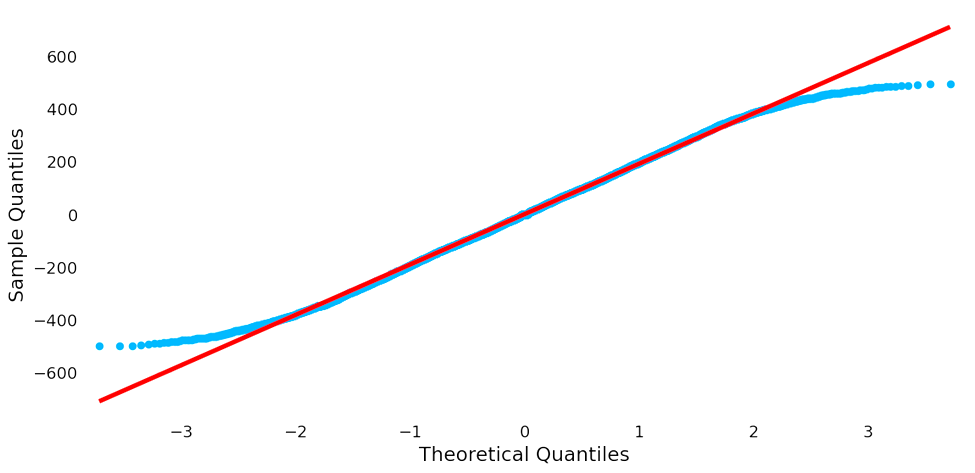
Figure 1. Result of Q-Q plot (Figure Credits: Original).

3.2. Result of Linear Regression

The model is predicted by linear regression and indicates the predictor (Y) is profit and variable (X) is discount, sales and region have a linear relationship. Performances are shown in Figure 2, which would also be similar to the expectation based on the Quantile-Quantile plot. The code uses Plotly to create a scatter plot. the x-axis represents the actual values, and the y-axis represents the model predictions. The scatterplot allows you to visualize the predictions of the model. The plot includes two lines, one where the predicted values are equal to the actual values, and the other is the model's prediction.

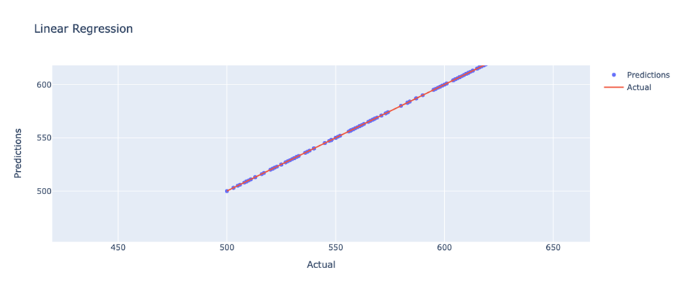
Figure 2. Result of linear regression (Figure Credits: Original).

3.3. Result of Polynomial Regression

A Polynomial Features object is created, transforming the original features into polynomial features for the specified number of times. The use of degree=2 indicates that the features are converted to quadratic polynomials. Compared to linear regression, polynomial regression improves the model fit by converting features to quadratic polynomials. The results show a perfect fit of the polynomial regression model on this dataset, with an MSE close to zero and an R² of 1.0, indicating that the model fits the data almost perfectly. More side-by-side comparisons were also made. Adjust the degree to 3, 4, and 5. Table 2 shows a portion of the data results.

All of these variations of the degree can be represented as performing very well on the training set, fitting the data almost perfectly. When analyzed from an MSE perspective, smaller values indicate that the difference between the model's predicted and actual values is more negligible, and therefore, the model performs better.

Table 2. Result of polynomial regression.

The complexity of the model should also be considered. In polynomial regression, as the number of polynomials increases, the complexity of the model also increases, which may lead to overfitting. Therefore, an appropriate model complexity must be chosen case-by-case to balance the fitting and generalization capabilities. An overfitted model "remembers" the data details too well in the training set, resulting in poor generalization to new data.

3.4. Result of Ridge Regression

The alpha values are 0.1, 1.0, and 10.0 in the regression model used in the experiments. To select the optimal alpha value in ridge regression using cross-validation to evaluate the model's performance and to select the optimal hyperparameters. After comparison, it is found that alpha = 0.1 is the best regularization parameter selected by cross-validation.

3.5. Result of Logistic Regression

The data selected through the experiment has a certain continuity and is unsuitable as an object of logical recursion. Results are shown in Figure 3. The research would also test the continuity data for logical recursion to check if predicting the profit is possible. In that case, this work gets icons that don't fit expectations and a negative R².

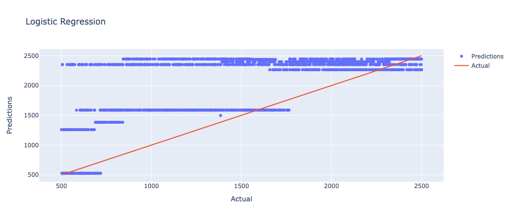
Figure 3. Result of logistic regression (Figure Credits: Original).

3.6. Result Comparison

The following MSE and R² in Table 3 are taken for the best case of each regression experiment for comparison.

Table 3. Result comparison.

After sorting through the models and comparing the models using MSE and R² as metrics, Linear Regression, Polynomial Regression, and Ridge Regression, all perform approach to perfect, with R² very close to 1.0 and MSE values very close to zero. Logistic Regression performs relatively poorly. the MSE is very high, and the R² is negative, which may indicate that the model does not apply to the problem. In summary, the linear regression, polynomial regression, and ridge regression models all performed very well on this particular dataset. They could be considered a suitable model.

4. Discussion

The dataset selection may influence the conclusions. For example, the dataset may only include order information for a specific period. More historical data may be needed if a long-term trend analysis or study of seasonal variations is required. The address information may only include regions without providing more detailed geographic location information, thus preventing more granular geographic analysis. To predict the accurate experiments of the model, more data are needed for validation analysis.

The present study is analyzed and discussed only in the Tamil Nadu, India dataset. However, profit as a complex link exists in social and business use. The economic level and development of the region are closely linked to shopping capacity and market development. Supply chain management forecasting must be adjusted according to the local economic level for better application in more scenarios.

5. Conclusion

These models can help companies understand the relationship between various links in the supply chain and make predictions and decisions based on historical data. For example, these models can be used to optimize inventory management, improve delivery punctuality, and develop production plans. Specifically, linear regression is more practical for analyzing the impact of a single variable on a target metric, such as analyzing the relationship between sales volume and promotional activities and the relationship between transportation time and delivery on-time rate. In contrast, polynomial regression better fits non-linear relationships. Final ridge regression deals with datasets with multiple covariates, for example, by simultaneously considering the impact of different supply chain segments on inventory levels and their interrelationships. A more accurate judgment is made on the forecasting of the supply chain.

References

[1]. Ng, I. C., & Wakenshaw, S. Y. (2017). The Internet-of-Things: Review and research directions. International Journal of Research in Marketing, 34(1), 3-21.
[2]. Yang, Z., Van Ngo, Q., Chen, Y., Nguyen, C. X. T., & Hoang, H. T. (2019). Does ethics perception foster consumer repurchase intention? Role of trust, perceived uncertainty, and shopping habit. Sage Open, 9(2), 2158244019848844.
[3]. Supermart Grocery Sales - Retail Analytics Dataset, URL: https://www.kaggle.com/datasets/mohamedharris/supermart-grocery-sales-retail-analytics-dataset. Last Accessed: 2023/09/27
[4]. Janiesch, C., Zschech, P., & Heinrich, K. (2021). Machine learning and deep learning. Electronic Markets, 31(3), 685-695.
[5]. Mahesh, B. (2020). Machine learning algorithms-a review. International Journal of Science and Research, 9(1), 381-386.
[6]. Su, X., Yan, X., & Tsai, C. L. (2012). Linear regression. Wiley Interdisciplinary Reviews: Computational Statistics, 4(3), 275-294.
[7]. Ostertagová, E. (2012). Modelling using polynomial regression. Procedia Engineering, 48, 500-506.
[8]. McDonald, G. C. (2009). Ridge regression. Wiley Interdisciplinary Reviews: Computational Statistics, 1(1), 93-100.
[9]. LaValley, M. P. (2008). Logistic regression. Circulation, 117(18), 2395-2399.
[10]. Sperandei, S. (2014). Understanding logistic regression analysis. Biochemia medica, 24(1), 12-18.
Cite this article
Lu,X. (2024). A comparative study of machine learning-based regression models for supply chain management. Applied and Computational Engineering,53,48-55.
Data availability
The datasets used and/or analyzed during the current study will be available from the authors upon reasonable request.
Disclaimer/Publisher's Note
The statements, opinions and data contained in all publications are solely those of the individual author(s) and contributor(s) and not of EWA Publishing and/or the editor(s). EWA Publishing and/or the editor(s) disclaim responsibility for any injury to people or property resulting from any ideas, methods, instructions or products referred to in the content.
About volume
Volume title: Proceedings of the 4th International Conference on Signal Processing and Machine Learning
© 2024 by the author(s). Licensee EWA Publishing, Oxford, UK. This article is an open access article distributed under the terms and
conditions of the Creative Commons Attribution (CC BY) license. Authors who
publish this series agree to the following terms:
1. Authors retain copyright and grant the series right of first publication with the work simultaneously licensed under a Creative Commons
Attribution License that allows others to share the work with an acknowledgment of the work's authorship and initial publication in this
series.
2. Authors are able to enter into separate, additional contractual arrangements for the non-exclusive distribution of the series's published
version of the work (e.g., post it to an institutional repository or publish it in a book), with an acknowledgment of its initial
publication in this series.
3. Authors are permitted and encouraged to post their work online (e.g., in institutional repositories or on their website) prior to and
during the submission process, as it can lead to productive exchanges, as well as earlier and greater citation of published work (See
Open access policy for details).