1. Introduction

The exploration of power amplifier linearization technology dates back to the 1920s. Traditional linearization technologies, such as feedforward technology, feedback technology, and analog predistortion technology, emphasize compensating power amplifier distortion through circuit design in the analog domain [1].

The feedforward method operates on the principle of separately extracting the distorted component of the power amplifier output signal. This distorted signal is then coupled with the output signal. When the amplitude of the distorted signal equals that of the distorted component in the output signal and they are opposite in phase, the distorted signal can neutralize the distorted component in the power amplifier output signal. While feedforward technology finds application in broadband scenarios, it presents challenges. It demands high precision in controlling the delay, amplitude, and phase to meet linearization requirements, resulting in complexity, high hardware costs, and substantial power consumption.

Contrastingly, the feedback method is apt for narrow bandwidth scenarios but falls short for broadband predistortion. In an analog predistortion system, a predistorter module, set before the power amplifier, introduces an opposite distortion. Despite this counteractive approach, the efficacy of analog predistortion linearization remains suboptimal, and it can process only a limited signal broadband. As shown in Figure 1, 2 and 3.

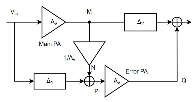
Figure 1. Feed forward technology schematic (Photo/Picture credit: Original).

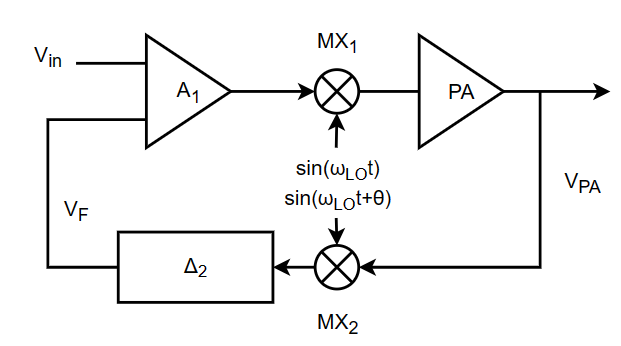
Figure 2. Feedback technique diagram (Photo/Picture credit: Original).

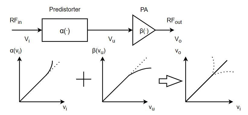
Figure 3. Analog predistortion (Photo/Picture credit: Original).

1.1. Emergence of digital predistortion technology

Upon crossing into the 21st century, the character of communication signals began a marked transformation, transitioning from narrowband constant envelope signals to wideband non-constant envelope signals. This evolution rendered traditional power amplifier linearization technology facing a significant application bottleneck. In response to this challenge, researchers have put forth highly efficient power amplifier architectures, such as class-E, class-F, envelope tracking technology, and outphasing technology among others. Amidst these innovations, the advent of digital predistortion technology marked a pivotal breakthrough. When juxtaposed with analog predistortion, digital predistortion technology stands out with conspicuous advantages. It boasts of high compensation precision, expansive compensation broadband, and a more versatile adaptation to various power amplifiers. These inherent benefits position digital predistortion technology as a forward-thinking solution, adept at navigating the complex demands of modern communication systems and ensuring the seamless, high-quality transmission of wideband non-constant envelope signals.

1.2. Early stages of development

In the early stage of the development of this technology, the model of digital predistorter is mainly constructed through lookup table and nonlinear behavior modeling. In the lookup table, the amplifiers' amplitude and phase responses are recorded as a function of the input power, and these responses are inverted to ensure the linearization function of the predistorter. In pre-distortion operation, the input signal power is used as the address index, and the unique amplitude-phase information is obtained by looking up the table. According to different construction, there are three types of predistorter structures based on lookup table: mapping structure, compound gain structure and polar coordinate structure.

Predistorters based on mapping structure requires two two-dimensional lookup tables. In this structure, the two orthogonal I and Q signals are input, and the output of the two lookup tables correspond to the I or Q pre-distorted signals, respectively. In a compound gain structure, a one-dimensional lookup table is used to search according to the power value of the input signal and output the compound gain required by the pre-distorted signal.

1.3. 21st Century

After entering the 21st century, people's demand for communication is not limited to voice calls, but more to data services.

1.3.1. Nonlinear modeling with linear memory

Linear memory effect can be described by linear filter. According to the model structure, the models of power amplifier or predistorter are classified into two boxes, three boxes and parallel cascade models. Typical two-box model structures include Wiener model and Hammerstein model [2, 3]. As shown in Figure 4.

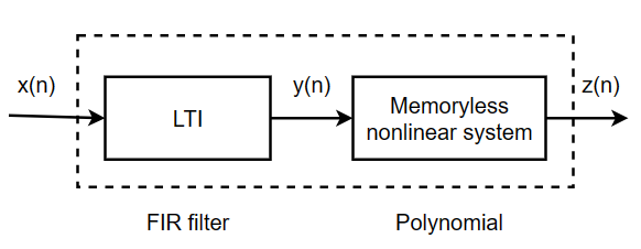
Figure 4. Diagram of the Wiener model (Photo/Picture credit: Original).

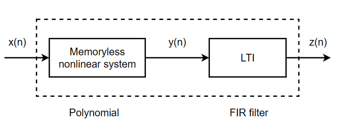
Figure 5. Diagram of the Hammerstein model (Photo/Picture credit: Original).

A typical three-box model is the Wiener-Hammerstein structure [4]. As shown in Figure 5 and 6.

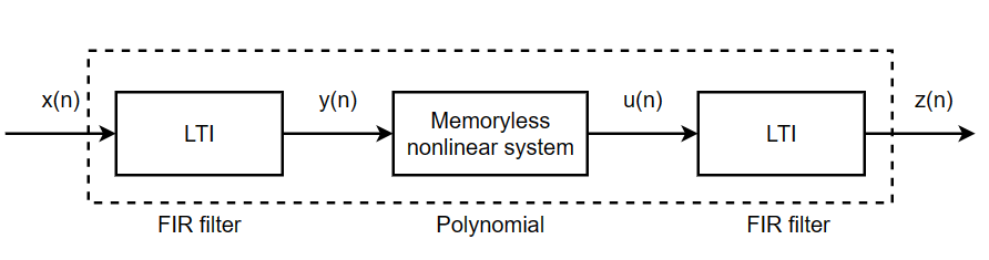
Figure 6. Diagram of the Wiener-Hammerstein model (Photo/Picture credit: Original).

1.3.2. Nonlinear modeling with nonlinear memory

In the two-box and three-box models, the description of memory effect and static nonlinearity is separated, which makes such models simple in structure and low in complexity. However, the existence of nonlinear memory effect is the normal distortion of power amplifier behavior under broadband excitation. Neural networks (NN) can also be used to construct nonlinear systems because NN can approximate any continuous function [5].

1.4. 2008-2016

With the development of 4G technology, some core wireless communication technologies have gradually flowed from academia to industry, helping users get a more rapid and reliable communication experience. But many problems have arisen.

Due to the scarcity of frequency resources, fragmentation of the wireless communication spectrum has become the norm. It is necessary to propose a suitable dual-frequency/multi-frequency digital predistortion technology. It needs a high-performance compensation scheme for the distortion characteristics of multi-channel transmitters. The acquisition and processing of wideband signal distortion increases the computational overhead and hardware cost of digital predistortion technology.

The distortion characteristics of the new high-efficiency amplifier architecture are more complex, and the pre-distortion algorithm and model performance can no longer apply to the current scenario.

2. Behavior characteristics of power amplifier

Power Amplifier (PA) is usually treated as a black-box model in digital predistortion technology.

The AM/PM effect will lead to system group delay distortion, differential gain, differential phase and intermodulation distortion, especially for the phase-sensitive systems such as frequency modulation and phase modulation signal systems. As a result, the bit error rate of the communication system increases.

The thermal memory effect is due to the heat generated by the operation of the power amplifier. This heat will affect the temperature sensitive power amplifier components, which will lead to a change in the performance of the power amplifier and make the power amplifier have a memory effect. Typically, thermal memory effects change more slowly and are considered long-term memory effects.

2.1. Amplifier behavior model

2.1.1. Power amplifiers without memory effects: lookup tables

Accordingly, the main feature of the memoryless effect model is that the input and output are in a one-to-one correspondence relationship up to the saturation point.

The predistorter based on the mapping structure requires two two-dimensional look-up tables. The inputs to the lookup table are two orthogonal I/Q input signals, respectively. The outputs of the two lookup tables correspond to the required I-way or Q-way predistorted signals, respectively.

The predistorter based on the polar structure requires two 1D look-up tables. The input to the phase lookup table is the amplitude signal of the predistorted signal. The predistorter based on complex gain requires a one-dimensional lookup table. In addition to lookup tables, typical nonlinear models are Saleh models. It was originally used to fit AM-AM characteristics and AM-PM characteristics of TWTS. In fact the fidelity of this model can barely meet the requirements of current behavior modeling, but Saleh model is still used as a power amplifier in numerical simulation.

2.1.2. Power amplifiers with memory effects: Volterra series and simplified polynomial models

In theory, Volterra series can be used to model any nonlinear system with memory. Because when the system has strong nonlinearity, it needs high-order Volterra series to fit. With the increase of the order, the correlation will become stronger, and the condition number of the regression matrix formed by the basis functions will become larger, which will lead to the numerical instability of the solution and the decline of the modeling accuracy. At the same time, too high order may also cause the model to overfit. In practical engineering applications, it is usually necessary to simplify the Volterra series to reduce the number of parameters and the amount of calculation, so as to achieve smaller hardware overhead and facilitate engineering implementation.

Due to its compact structure and low complexity, MP model has become the most common behavior model in the field of digital predistortion.

Denote the input of PA as z(n) and the output as y(n). The MP model can be written as follows.

\( {y_{MP}}(n)=\sum _{k=1}^{K}\sum _{q=0}^{Q-1}{a_{kq}}z(n-q){|z(n-q)|^{k-1}} \) (1)

Here, K is the order of the amplifier. K is always odd, which shows the amplitude distortion of PA.

\( {y_{GMP}}(n)=\sum _{K=1}^{{K_{a}}}\sum _{q=0}^{{Q_{a}}-1}{a_{kq}}x(n-q){|x(n-q)|^{k-1}} \) \( =+\sum _{k=1}^{{K_{b}}}\sum _{q=0}^{{Q_{b}}-1}\sum _{g=1}^{{G_{b}}}{b_{kq}}x(n-q){|x(n-q-g)|^{k-1}} \) \( =+\sum _{k=1}^{{K_{c}}}\sum _{q=0}^{{Q_{c}}-1}\sum _{g=1}^{{G_{c}}}{c_{kq}}x(n-q){|x(n-q+g)|^{k-1}} \) (2)

Here, \( {a_{kq}} \) , \( {b_{kq}} \) , and \( {c_{kq}} \) are the calculated nonlinear coefficients, and G represents the length of the cross-term. Compared with MP model, GMP model has more coefficients and is more complex.

2.2. Basic principles of digital predistortion

Predistortion techniques usually use some modeling algorithm to find the inverse system of the power amplifier, and the inverse system is realized by some circuit. As shown in Figure 7.

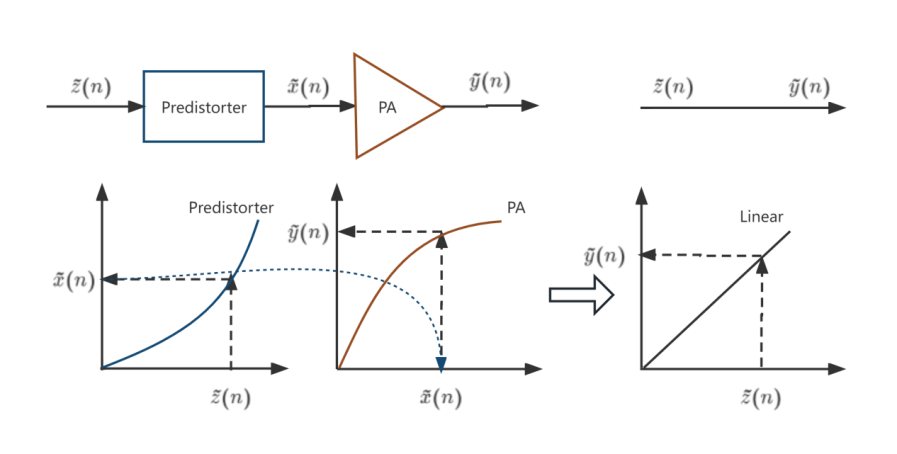
Figure 7. Structure diagram (Photo/Picture credit: Original).

2.3. Learning structure for digital predistortion

2.3.1. Indirect learning structure

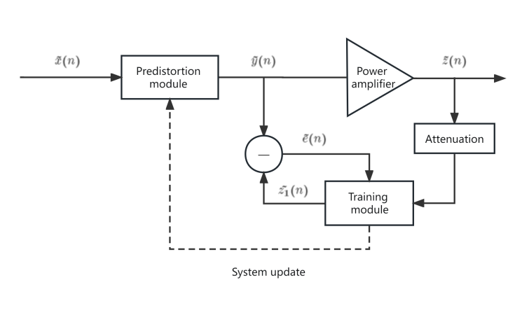
Figure 8. Structure diagram (Photo/Picture credit: Original).

The core concept of the predistorter hinges on acting as the preinverse of the system. Despite its utility, the approach is not without flaws. The indirect predistortion structure, tasked with obtaining the post-inverse of the power amplifier, encounters challenges. As shown in Figure 8. As the signal is fed back from the output of the power amplifier, noise is introduced following downconversion and AD conversion, compromising the linearity of the output signal post-predistortion. This limitation becomes markedly pronounced when the power amplifier enters a deep saturation region. Amid substantial nonlinear distortion, the efficacy of digital predistortion, employing an indirect learning architecture, witnesses significant degradation.

2.3.2. Direct learning structure

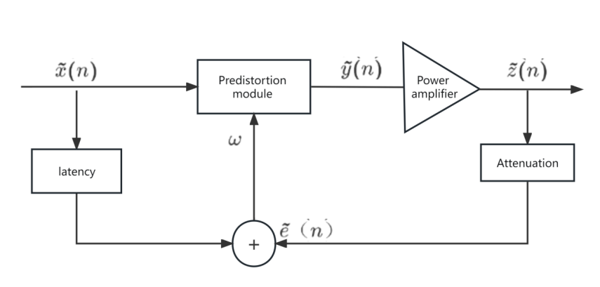
Figure 9. Structure diagram (Photo/Picture credit: Original).

The core concept of the direct learning architecture focuses on identifying the pre-inverse of the power amplifier [6]. When comparing the two modeling algorithms, considering the power amplifier as a nonlinear mapping, and assuming a one-to-one correspondence between the input and output of this mapping, the inverse of this mapping is unique, and the forward inverse is equal to the backward inverse. This scenario implies that two distinct inputs to a power amplifier may yield the same output. As shown in Figure 9. In this case, the input and output of the power amplifier no longer adhere to the one-to-one mapping relationship, and the post-inverse and pre-inverse of the power amplifier will no longer coincide.

2.3.3. Iterative learning control structure

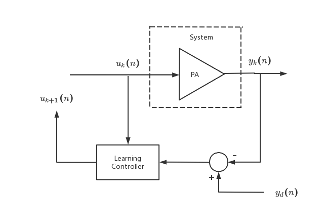
Figure 10. Structure diagram (Photo/Picture credit: Original).

As shown in Figure 10. In the process of approximating the best predistorted signal, the same signal needs to be continuously adjusted and input into the PA repeatedly, which means that the ILC structure cannot be applied in real time. However, the advantage of this architecture is that the computational complexity is low and only the addition, subtraction, multiplication and division operations are needed.

2.4. Parameter extraction algorithm for polynomial models

After the digital predistortion technology determines the predistortion model with high precision and meets the requirements, it is necessary to further determine the parameters of the predistortion model. Power amplifier is easily affected by the environment and device aging, which leads to the change of its nonlinear characteristics.

\( z(n)=\sum _{ \begin{array}{c} k=1 \\ k odd \end{array} }^{K}\sum _{q=0}^{Q}{a_{kq}}x(n-q){|x(n-q)|^{k-1}} \) (3)

\( {u_{kq}}(n)=y(n-q){|y(n-q)|^{k-1}} \) (4)

Write the above equation in matrix form:

\( z=Ua \) \( U=[{u_{10}},\cdot \cdot \cdot ,{u_{K0}},\cdot \cdot \cdot ,{u_{1Q}},\cdot \cdot \cdot ,{u_{KQ}}], \) \( {u_{kq}}={[{u_{kq}}(0),\cdot \cdot \cdot ,{u_{kq}}(N-1)]^{T}}, \) \( a={[{a_{10}},\cdot \cdot \cdot ,{a_{KO}},\cdot \cdot \cdot ,{a_{1Q}},\cdot \cdot \cdot ,{a_{KQ}}]^{T}} \) (5)

Although each term in a polynomial model is nonlinear, it has a linear response with respect to its coefficients.

2.4.1. LS algorithm

\( \hat{a}=({U^{H}}U{)^{-1}}{U^{H}}z \) (6)

LS algorithm is widely used in engineering because it does not need iteration, has low computational complexity and high solution accuracy. But LS has limitations. One is that LS algorithm needs to invert matrix \( {U^{H}}U \) in the process of parameter extraction. Second, when matrix \( {U^{H}}U \) is singular matrix, LS algorithm can not calculate the inverse.

2.4.2. LMS algorithm

LMS is a common adaptive filtering algorithm. It is based on a simple linear model, and iteratively adjusts the model parameters to minimize the sum of squared prediction errors, so as to gradually approximate the true model of the signal.

\( w(n+1)=w(n)+μ\cdot e(n)x(n) \) \( R(n)=d(n)-y(n) \) (7)

Among them, the w(n) refers to the model parameters at time n. \( μ \) is the learning rate, also called the step size. It determines the update amount of model parameters in each iteration and affects the convergence speed of the algorithm. R(n) refers to the actual output signal. Y (n) refers to the deviating from the expected output d(n). x(n) refers to the current input signal.

3. Cutting edge technology for digital predistortion

3.1. Neural networks

Neural network has a strong ability of nonlinear fitting, so it can model the behavior of power amplifier. The existing GMP model performs well in the narrow band range, but its linearization ability decreases as the signal bandwidth increases. In the future, neural networks will be a powerful means to solve the complex nonlinear distortion of future Ultra-wide Bandwidth (UWB) transmitters.

3.1.1. Real-valued Delayed Neural Networks: RVTDNN [7]

The neural network mimics the time delay through multiple unit delay operators. The total delay is the memory depth of the system. Each neuron (the basic building block of A neural network) has its weight \( ω_{nj}^{l} \) and bias \( b_{n}^{l} \) . At any time \( k \) , the output of the NTH neuron in layer \( l \) is: \( net_{n}^{l}(k)=\sum _{j=1}^{N}ω_{nj}^{l}O_{j}^{l-1}(k)+b_{n}^{l} \) . \( N \) denotes the number of neurons in the corresponding layer. \( l \) denotes the number of layers and takes the values 1, 2, ..., L. As shown in Figure 11.

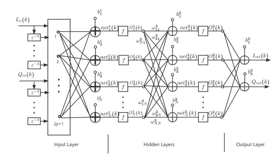
Figure 11. Schematic diagram (Photo/Picture credit: Original).

3.1.2. Time-delay neural network model based on vector decomposition: VDTDNN [8]

Since the I/Q channels are orthogonal and independent of each other, it is difficult for neural networks to accurately fit two nonlinear functions at the same time. Only the modulus value of the input signal is operated nonlinearly. Where \( {θ_{n-m}} \) is the phase information of input signal \( x(n-m) \) . \( h \) is the output \( O_{g}^{L-1} \) of the last hidden layer in VDTDNN, and it is only related to the modulus value of the input signal. At the same time, the last hidden layer needs to enter the PRB unit for phase recovery after passing through the fully connected layer, and then obtain the output of the I/Q two channel signals. As shown in Figure 12.

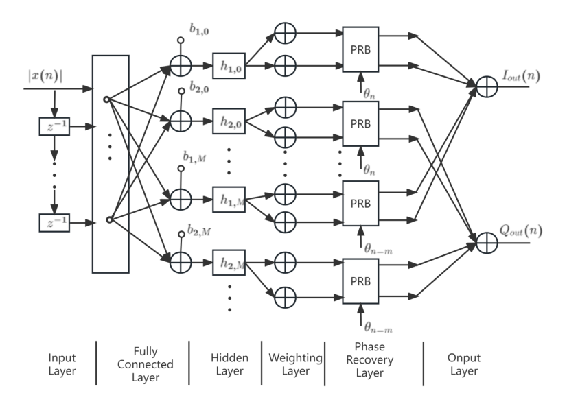
Figure 12. Neural network diagram (Photo/Picture credit: Original).

3.2. MIMO

With the augment of MIMO transmitter system integration, DPD model mismatch caused by crosstalk effect between transmitting links decreases the traditional DPD linearization performance. With the increase of nonlinear characteristics and memory effect of power amplifier devices, the complexity of DPD model increases, the computation and implementation cost of predistorter increase, then the efficiency of the system reduced.

The improvement of these problems is mainly carried out from two aspects: architecture and anti-nonlinear crosstalk technology.

3.2.1. Research on DPD architecture of MIMO system

Considering the use of single digital stream and single beam, the RF link including space propagation can be simplified into a nonlinear system with single input and single output, which makes it possible to simplify the modeling of array system and its DPD architecture. Based on this, researchers such as M. Abdelaziz from Tampere University of Technology in Finland and Professor Chen Wenhua's research group from Tsinghua University in China put forward Beam-Oriented digital predistortion technology (BO-DPD) nearly at the same time [9]. The advantage of BO-DPD is that it uses only a traditional single predistortion module to linearize the signal in the main beam, and the architecture is extremely simple. However, the problem is that the modified architecture can only achieve linearization in a single direction. However, there are spatial nonlinear leakage in other azimuths.

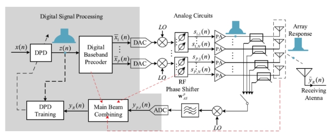
Figure 13. Diagram of BO-DPD Structure (Photo/Picture credit: Original).

As shown in Figure 13. To address this issue, Professor Yu Chao from Southeast University introduced the Full-Angle DPD technology [10]. This advanced technology, built upon the foundation of BO-DPD, employs a cascading structure. By incorporating Tuning boxes, it compensates for the nonlinear discrepancies of each link, thereby ensuring the output of each power amplifier is effectively linearized.

3.2.2. Research on anti-nonlinear crosstalk technology

In light of future transmitter systems’ constraints on size, power consumption, weight, cost, and complexity, forthcoming massive MIMO arrays will forego the use of isolators or circulators in the power amplifier output. This exclusion will lead to the mutual coupling between antenna elements, introducing nonlinear crosstalk and impacting the overall efficacy of the DPD system.

A notable advancement to counter this is the Cross-talk cancelling DPD, proposed by P. Suryasarman et al., from Johannes Kepler University in Austria [11]. This approach eradicates preamplifier crosstalk by employing linear elimination directly preceding the power amplifier. Through the DPD model coefficient extraction process, it enables the estimation of the coupling coefficient, contributing significantly to enhancing the system's performance by mitigating the adverse effects of crosstalk. As shown in Figure 14.

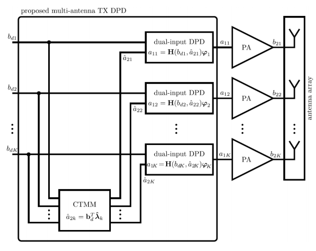
Figure 14. Diagram of DI-CTMM DPD model (Photo/Picture credit: Original).

Based on the DI-CTMM DPD model, the group led by Professor Hong Wei at Southeast University crafted a dual-input model. This advancement was made by incorporating a normalized piecewise linear CPWL function and DVR model to enhance the linearization performance of the DI-CTMM DPD [12, 13]. This refined model adeptly strikes a balance, successfully reducing model complexity while adeptly handling high-order nonlinear crosstalk, thus significantly improving overall linearization performance.

3.2.3. Piecewise linear CPWL function

\( {f_{0}}(n)=\sum _{i=0}^{M}{c_{i,1}}{a_{1k}}[n-i] \) \( {f_{21}}(n)=\sum _{r=1}^{R}\sum _{i=1}^{M}{c_{ri,21}}||{a_{1k}}[n-i]|-{β_{r}}|{a_{1k}}[n-i]|{a_{1k}}[n]| \) \( {f_{22}}(n)=\sum _{r=1}^{R}\sum _{i=1}^{M}{c_{ri,22}}||{a_{1k}}[n-i]|-{β_{r}}|{a_{1k}}[n] \) \( {f_{23}}(n)=\sum _{r=1}^{R}\sum _{i=0}^{M}{c_{ri,23}}||{a_{1k}}[n-i]|-{β_{r}}|{a_{1k}}[n-i] \) \( {f_{24}}(n)=\sum _{r=1}^{R}\sum _{i=1}^{M}{c_{ri,24}}||{a_{1k}}[n]|-{β_{r}}|{a_{1k}}[n-i] \) (8)

3.2.4. DVR model

\( {F_{0}}(n)=\sum _{i=0}^{M}{c_{i,2}}{a_{2k}}[n-i] \) \( {F_{21}}(n)=\sum _{r=1}^{R}\sum _{i=0}^{M}{c_{ri,31}}||{a_{2k}}[n-i]|-{β_{r}}|{a_{2k}}[n-i]|{a_{1k}}[n]| \) \( {F_{22}}(n)=\sum _{r=1}^{R}\sum _{i=0}^{M}{c_{ri,32}}||{a_{2k}}[n-i]|-{β_{r}}|{a_{1k}}[n] \) \( {F_{23}}(n)=\sum _{r=1}^{R}\sum _{i=0}^{M}{c_{ri,33}}||{a_{1k}}[n-i]|-{β_{r}}|{a_{2k}}[n-i] \) \( {F_{24}}(n)=\sum _{r=1}^{R}\sum _{i=1}^{M}{c_{ri,34}}||{a_{1k}}[n]|-{β_{r}}|{a_{2k}}[n-i] \) \( {F_{25}}(n)=\sum _{r=1}^{R}\sum _{i=0}^{M}{c_{ri,35}}||{a_{1k}}[n]|-{β_{r}}|a_{1k}^{2}[n]a_{2k}^{*}[n-i] \) (9)

4. Conclusion

Over more than three decades of advancement, various factors have propelled the continuous improvement and optimization of predistortion technology. The expansion of signal bandwidth, the consistent increase of memory components in the signal, the scarcity of frequency resources, and the advent of multi-channel transmitters have all played a significant role in this evolution. Predistortion technology has transformed from the analog to the digital domain, with the proposal of nonlinear modeling models that include memory. Comprehensive research has been conducted on the dual-frequency/multi-frequency parallelization of RF power amplifiers, multi-channel MIMO transmitters, and the linearization of dual-input high-efficiency power amplifiers. In today's 5G era, the integration of this technology with neural networks and deep learning marks a novel and promising direction of research.

Authors Contribution

All the authors contributed equally and their names were listed in alphabetical order.

References

[1]. Katz, A., Wood, J., & Chokola, D. (2016). The evolution of PA linearization: from classic feedforward and feedback through analog and digital predistortion. IEEE Microwave Magazine, 17, 32-40.
[2]. Kang, H. W., Cho, Y. S., & Youn, D. H. (1998). Adaptive precompensation of Wiener systems. IEEE Transactions on Signal Processing, 46, 2825-2829.
[3]. Ding, L., Raich, R., & Zhou, G. T. (2002). A Hammerstein predistortion linearization design based on the indirect learning architecture. Proceedings of the IEEE International Conference on Acoustics, Speech, and Signal Processing (pp. 2689-2692). IEEE.
[4]. Tan, A. H. (2006). Wiener-Hammerstein modeling of nonlinear effects in bilinear systems. IEEE Transactions on Automatic Control, 51, 648-652.
[5]. Eun, C., & Powers, E. J. (1997). A new Volterra predistorter based on the indirect learning architecture. IEEE Transactions on Signal Processing, 45(1), 223-227.
[6]. Braithwaite, R. N., & Carichner, S. (2009). An Improved Doherty Amplifier Using Cascaded Digital Predistortion and Digital Gate Voltage Enhancement. IEEE Transactions on Microwave Theory and Techniques, 57(12), 3118-3126.
[7]. Chani-Cahuana, J., Landin, P. N., Fager, C., & Eriksson, T. (2016). Iterative Learning Control for RF Power Amplifier Linearization. IEEE Transactions on Microwave Theory and Techniques, 64(9), 2778-2789. https://doi.org/10.1109/TMTT.2016.2588483
[8]. Liu, T., Boumaiza, S., & Ghannouchi, F. M. (2004). Dynamic behavioral modeling of 3G power amplifiers using real-valued time-delay neural networks. IEEE Transactions on Microwave Theory and Techniques, 52(3), 1025-1033.
[9]. Zhang, Y., Li, Y., Liu, F., & Zhu, A. (2019). Vector Decomposition Based Time-Delay Neural Network Behavioral Model for Digital Predistortion of RF Power Amplifiers. IEEE Access, 7, 91559-91568. https://doi.org/10.1109/ACCESS.2019.2927875
[10]. Liu, X., Zhang, Q., Chen, W., et al. (2018). Beam-Oriented Digital Predistortion for 5G Massive MIMO Hybrid Beamforming Transmitters. IEEE Transactions on Microwave Theory and Techniques, 66(7), 3419-3432.
[11]. Yu, C., Jing, J., Shao, H., et al. (2019). Full-Angle Digital Predistortion of 5G Millimeter-Wave Massive MIMO Transmitters. IEEE Transactions on Microwave Theory and Techniques, 67(7), 2847–2860.
[12]. Suryasarman, P., Hoflehner, M., & Springer, A. (2013). Digital Pre-Distortion for Multiple Antenna Transmitters. 2013 European Microwave Conference (pp. 412-415). IEEE.
[13]. Hausmair, K., Landin, P. N., Gustavsson, U., et al. (2018). Digital Predistortion for MultiAntenna Transmitters Affected by Antenna Crosstalk. IEEE Transactions on Microwave Theory and Techniques, 66(3), 1524–1535.
Cite this article
Chen,B.;Wu,W. (2024). Principles, applications, and challenges of digital predistortion technology. Applied and Computational Engineering,54,64-75.
Data availability
The datasets used and/or analyzed during the current study will be available from the authors upon reasonable request.
Disclaimer/Publisher's Note
The statements, opinions and data contained in all publications are solely those of the individual author(s) and contributor(s) and not of EWA Publishing and/or the editor(s). EWA Publishing and/or the editor(s) disclaim responsibility for any injury to people or property resulting from any ideas, methods, instructions or products referred to in the content.
About volume
Volume title: Proceedings of the 4th International Conference on Signal Processing and Machine Learning
© 2024 by the author(s). Licensee EWA Publishing, Oxford, UK. This article is an open access article distributed under the terms and
conditions of the Creative Commons Attribution (CC BY) license. Authors who
publish this series agree to the following terms:
1. Authors retain copyright and grant the series right of first publication with the work simultaneously licensed under a Creative Commons
Attribution License that allows others to share the work with an acknowledgment of the work's authorship and initial publication in this
series.
2. Authors are able to enter into separate, additional contractual arrangements for the non-exclusive distribution of the series's published
version of the work (e.g., post it to an institutional repository or publish it in a book), with an acknowledgment of its initial
publication in this series.
3. Authors are permitted and encouraged to post their work online (e.g., in institutional repositories or on their website) prior to and
during the submission process, as it can lead to productive exchanges, as well as earlier and greater citation of published work (See
Open access policy for details).