1. Introduction

As early as many years ago, people began to carry out technical research on Simultion Localization and Mapping (SLAM). Today, with the significant increase in computer processing speed and the popularization of low-cost sensors such as cameras and laser rangefinders, SLAM is being put into practical use in more and more fields.

SLAM or Simulation Localization and Mapping is the algorithm tool that helps robot build the surrounding unknow map and localize its location within the map that has been constructed through the complex data process. It is widely used in the autonomous vehicle that can achieve the route planning and automatic obstacle avoidance and it is a promising and potential future developing direction in the intelligent robot.

The SLAM algorithm has been taken widely in the area of autonomous intelligence more than two decades [1] and with the continuing development, the scientists use this technique to improve the intelligent robot in navigation capacity. Since there are many different SLAM methods for different goals, it is not easy to compare them. Choosing the most appropriate approach for a particular application requires a good knowledge of the ins and outs of SLAM, as well as a global understanding of state-of-the-art SLAM strategies. The performance of the method depends on the application context and the challenge to be solved. On a global scale, SLAM is often mistakenly thought of as a one-size-fits-all technology, but real-world implementations raise many questions about computational limitations, noise suppression, and even user-friendliness. It's just a choice of difficulties to overcome. It can be learned in the Zhang’s original work that the basic principle of LIDAR-based 3D SLAM technology [2] and owning to this work, the algorithm contributes to selecting and extracting the feature points information of effective edge and plane from complex point cloud. Through the integration calculator of the gyroscope and accelerometer of the six-axis Inertial Measurement Unit (IMU) to get the prior pose, improving the accuracy of LIDAR odometer, many LIADR-IMU loosely coupled systems were effectively furthered on the basis of SLAM.

To achieve SLAM algorithm, sensor signal processing and pose map optimization, two technologies including front-end processing and back-end processing, are needed. To learn more about front-end processing techniques, in this paper, there is a further explanation about SLAM method, named LIDAR SLAM.

LIDAR, used in LIDAR SLAM as sensor to localize and map, are increasingly applied in the intelligent robotics and vehicles and LIDAR SLAM is widely and deep researched to improve its accuracy and reliability [3]. However, it still remains challenges in dynamic and real-time scenarios.

Currently, there is some LIDAR SLAM frameworks achieve mapping and localization by extracting geometric features, for example the derivative algorithm of LIDAR Odometry And Mapping (LOAM) [2] [4], and HDL-Graph-SLAM [5], but they overlook the intensity information. In recent year, some LIDAR SLAMs based on high intensity are proposed, but most of works seriously rely on a prior intensity map of the testing area which is difficult to meet especially in large, unknown scale environment.

Before in-depth exploration the LIADR SLAM, it is helpful to preview the loosely coupled system. The appearance of loosely coupled system innovated the multi-sensor fusion system and widely used in the low-budget. The loosely coupled system is reflected in the low bandwidth of interconnection and small communication between nodes. It is the system that communication is executed by the way of information transfer and each node can successfully complete computer task respectively.

In most case, the LIDAR SLAM based on the LOAM, a framework that merged with SCAN-to-SCAN and SCAN-to-MAP modes, performs better than the visual SLAM [2]. What more, the loop closure detection techniques, based on the LIDAR, has been widely applied in the place recognition and graph optimization in order to decline the error caused by the LIDAR SLAM.

However, either standalone visual or LIDAR SLAM remains some currently unsolved problems. It is easy for visual SLAM to fail to orientate correct while moving fast [6]. On the other hand, as for LIDAR SLAM, it is complex for scientists to sole the motion distortion and due to lack for stable feature, it is more challenge and elaborate to perfect the closure loop detection [7]. Therefore, combining with these SLAM to improve the overall performance is the direction and tendency that deserves researchers to think carefully.

However, SLAM in this field has been researched for a long time and many studies covered are conducted. In this paper, it is organized to have further explanation and description in the LIDAR SLAM and its optimal algorithm LOAM. It is meaningful to human intelligence and usefully obtaining the high accuracy distance measurement data, provided by LIDAR sensor points cloud and SLAM constructing. Of course, the process to achieve SLAM algorithm is much more complex which includes probability theory, state estimation, optimization theory, perceptual fusion and so on.

To achieve the application of SLAM working, the LOAM algorithm can be a good tool to make optimization. It takes Lidar registration and Odometry and Mapping as core. After extracting features, the coarse positioning can be made by the high frequency odometry and accurate positioning by low frequency odometry. LOAM algorithm uses a known clous sequence by scanning to calculate radar poses in the first K periods and construct the global map. What’s more, the radar pose is estimated by the attitude change relationship between adjacent frames and to reduce computation and calculation time, it usually chooses to use feature point in cloud points. And it is a suitable choice to use curvature of a point to compute plane smoothness as the index ofg present feature information [2].

This paper is organized to introduce the application of SLAM algorithm and further improvement in LOAM algorithm in ocean autonomous robot. It will begin with the basic principle, structure, feature and the process overview of SLAM. After this, the advantages and challenges will be covered and the LOAM algorithm will be introduced and stated how it can improve the algorithm.

2. Method

2.1. Simultaneous Localization and Mapping System

SLAM systems that utilize a range of sensors, including LIDAR, cameras, radar, and others, have seen significant development over the past decade. The concept of a feature-based fusion SLAM framework was first introduced in 1990 and remains relevant in current research and applications. It can be divided into two modules, mapping and localization. For the whole system, these two modules are combined, interact and promote each other. The system's operational principle relies on the reconstruction and stitching of three-dimensional scenes, facilitated by a high-precision odometer composed of multiple sensors. This odometer plays a crucial role in providing real-time attitude estimation for the robot. Simultaneously, achieving high-precision 3D reconstruction offers vital data for the feature-based odometer's attitude estimation. In any odometer system, the creation or storage of temporary local maps is essential to support attitude estimation.

2.2. Multi-Sensor System Based on LIDAR

The widespread adoption and interest in LiDAR-based 3D SLAM can be traced back to Zhang's pioneering work, specifically the LOAM algorithm [8]. Within intricate point cloud data, it effectively extracts edge and plane feature points, creating error functions based on point-to-line and point-to-plane distances to address the non-linear optimization challenge in attitude estimation

In Shan's 2018 paper [9], the Lightweight and Groud-Optimized Lidar Odometry and Mapping on Variable Terrain (LeGO-LOAM) algorithm was introduced, incorporating point cloud clustering and ground segmentation to enhance cloud registration during data processing. Additionally, it employed a straightforward acceleration function for IMU data processing, facilitating point cloud distortion correction and the provision of a prior pose. In the field of SLAM systems, single-sensor setups have matured, with LIDAR sensors being the most prevalent choice. However, data collected by a single sensor, while rich, tends to be discrete despite its ability to provide various environmental information. Therefore, leveraging multi-sensor systems based on LIDAR allows for the utilization of LIDAR and other complementary sensors to capture more detailed and accurate data.

2.3. 2D&3D LIDAR sensor system

The 2D LIDARs usually are used in the localization and mapping and when the scan rate is higher than the external moving rate, there may occur a motion distortion in the scan. In this case, an Iterative closet point (ICP) [10] method can be used to remove the distortion. It is using the computed velocity to achieve the distortion compensation step after the ICP based velocity estimation step. This method can still be used in the 3D LIDAR sensor system to compensate the distortion. However, if the rate of scan is much lower than the motion rate, the distortion may be severe especially in 2D LIDAR system because one axis is much slower than the other one. Next part is to introduce the 3D LIDAR and the ego-motion estimation based on point cloud.

2.4. Definition and Overview

We define the right subscription \( k, k∈{Z^{+}} \) to indicate a sweep in one time coverage and \( {P_{k}} \) represents the point cloud perceived during the sweep \( k \) . And two coordinates are defined, respectively are LIDAR coordinate system {L} and world coordinate system {W}. The origin of {L} is the geometric centre of LIDAR sensor and the x-axis points left, the y-axis points upward and z-axis points forward. The coordinates of a point \( i, i∈{P_{k}} \) in { \( {L_{k}} \) } can be expressed as \( X_{(k,i)}^{L} \) . And the {W} is similar to the {L} with the origin coincidence and the coordinates of \( i, i∈{P_{k}} \) can be expressed as \( X_{(k,i)}^{W} \) .

2.5. LIDAR Odometry

At the beginning, the feature points that are extract from Lidar cloud, are denoted as \( {P_{k}} \) . The Lidar system inherently produces a non-uniform distribution of points within \( {P_{k}} \) . The laser scanner's returns have a resolution of \( 0.25° \) within a single scan due to the rotational speed of \( 180°/s \) , resulting in scans being generated at 40Hz. Consequently, the resolution in the direction perpendicular to the scaning planes is \( 4.5° \) . Given this consideration, we extract feature points from \( {P_{k}} \) by utilizing information solely from individual scans, taking into account their co-planar geometric relationship. Specifically, we select feature points located on sharp edges and flat surface segments. Let \( i \) represent a point in \( {P_{k}}, i∈{P_{k}} \) , and let \( S \) represent the collection of sequential points obtained by the laser scanner within a single scan. As the laser scanner produces point returns either in a clockwise (CW) or counterclockwise (CCW) order, \( S \) comprises half of its points on each side of i with intervals of \( 0.25° \) between two points. We define a metric to assess the local surface's smoothness.

\( c=\frac{1}{|S|∙|X_{(k,i)}^{L}|}||\sum _{j∈S,j≠i}(X_{(k,i)}^{L}-X_{(k,j)}^{L})|| \) (1)

The points within a scan undergo sorting based on their \( c \) values, following which feature points are chosen based on the highest \( c \) values, referred to as edge points, and the lowest \( c \) values, referred to as planar points. In order to achieve an even distribution of feature points across the environment, we divide a scan into four equally-sized subranges. Each subrange can contribute a maximum of 2 edge points and 4 planar points. If the value of a point, represented as ' \( i \) ,' exceeds a predefined threshold, it can be categorized as an edge point; otherwise, it can be classified as a planar point. Furthermore, it is essential to ensure that the quantity of chosen points does not surpass the predetermined upper limit. It is worth noting that we have named the point cloud of this projection Pk, so on the k+1 scan, Pk and newly received Pk+1 will be used together for motion scanning

2.6. Pose calculation

During the process of scanning, the data got from the LIDAR scanning will be used model under the constant angular and linear velocities to get the LIDAR motion. The point cloud and other quantities we get from the LIDAR scan are input into the algorithm in Zhang’s paper [2] as inputs, and it will output the attitude transformation serving for the next mapping step.

2.7. LIDAR Mapping

In the LIDAR mapping stage, the method of extracting feature points is the same as above, but the number of feature points will be ten times as many as above. In order to find the corresponding relationship of feature points, the cloud point will be recorded on a map with the size of 10 cubic meters. We apply the obtained information to the Levenberg-Marquardt method [11] for robust fitting [12] to solve nonlinear optimization. To achieve a uniform distribution of points, a voxel mesh filter [13], the size of which is a 5cm cubic, is applied to downsize the point cloud, the size of which is a 5cm cube. It is important to highlight that the LIDAR's orientation concerning the map results from a combination of two transformations, and it operates at the same frequency as the LIDAR odometer.

3. Result

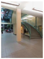
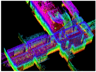
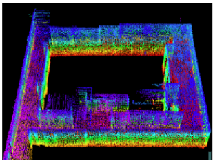
The LOAM in Ji Zhang and Sanjiv Singh’s paper [2] has been tested in both indoor and outdoor and the result showed all successful. In the indoor experiment, the LIDAR is placed in a small cart and experimenters pushed it in an indoor gallery and a lobby as the velocity of 5 meters per second. The figure 1(a) and 1(c) of environment, shown in the following, were shot by the experimenters and the maps figure 1(b) and 1(d) modelled by the LIDAR were similar and perfectly described the environment.

Similarly, in the outdoor experiment, the LIDAR was installed on the front of a vehicle and moving at 5 meters per second. The figure 2(b) and 2(d) which show pictures drew by the LIDAR can easily be seen that it is similar to the real environment shown by figure 2(a) and 2(c), which can prove that this text was reaching the expected aim.

What’s more, in the paper by Y. Su et al [14], they want to use LIDAR sensors to link the LOAM algorithm to perfect the ground rescue robot. And a complete perception system is built, and data sets in different environments are collected. Terrain conditions include long indoor corridors, outdoor roads, slopes, etc. It is worth noting that the IMU was used to optimize the open-source LOAM algorithm to improve its accuracy and the final result is shown in the figure 3 which shows well the structure of the terrain and it greatly helps the ground rescue robot adapt to a variety of different environments.

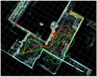
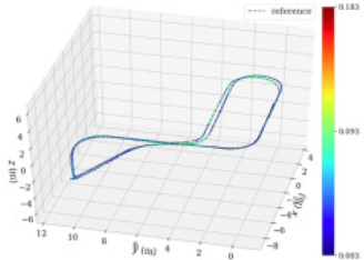
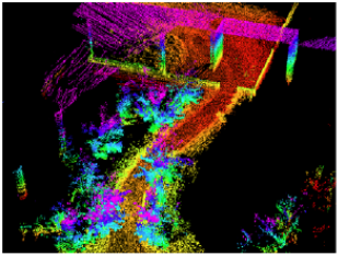
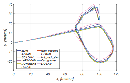
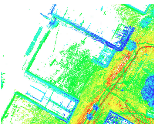
In a paper by Anton Koval et al. [15], it is mentioned that they want to use the SLAM algorithm of LiDAR to process the data collected by underground tunnels. According to their results shown in figure 4, although constructing terrain from underground tunnel data is a very challenging task, the radar-based SLAM algorithm can still successfully construct terrain using point clouds. Their results show that the LiDAR based SLAM algorithm, or LOAM algorithm, can be used to construct terrain and draw rough topographic maps in harsh environments where features are scarce.

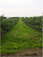
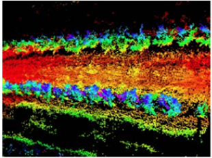
Besides, LOAM algorithm can be used in the agriculture field. It is known that there are significant differences between urban and agricultural landscape characteristics. Most of the agricultural scenes are plants such as trees and grass, and the features of the landscape such as grass and trees in the agricultural scenes are difficult to provide easy-to-detect features as the urban buildings. Therefore, T. Le. et al [16] wrote a paper related with the agricultural robots, equipped with the LOAM algorithm to map the complex agricultural environment. Although they compared the LOAM and their method and made a conclusion that the map built by their method was better than built by LOAM algorithm in some respects, the map figure 5 built by LOAM algorithm has more points in the picture and it is clearer.

On the other hand, this also shows that LOAM algorithm can be used in a wide range of applications, can be used in roads, narrow tunnels, and can also be used in agriculture-related scenarios.

4. Conclusion

The main findings of the paper are as follows: LOAM algorithm makes reasonable use of the characteristics of laser radar with high accuracy and strong feedback. At the same time, the obstacle features are transformed into point clouds, which is a clever method. The point clouds are characterized by 3D, sparsity and large amount of data to construct the terrain, and the automatic vehicle are well processed for terrain exploration and evaluation in unfamiliar environments. This method makes reasonable use of the advantages of scanning mode and point cloud distribution of Lidar, and carries out feature matching in the algorithm to ensure the rapidity and accuracy of the calculation. From the experimental results of the paper we discussed, LOAM algorithm is one of the SLAM algorithms that can solve terrain construction well. Although it does not have some advantages of other algorithms, it is still a competitive method with other algorithms.

References

[1]. Taheri H and Xia Z, Jan. 2021, “SLAM; definition and evolution,” ENG APPL ARTIF INTEL, vol. 97, p. 104032, doi: 10.1016/j.engappai.2020.104032.
[2]. Zhang J and Singh S, 12–14 July 2014, “LOAM: Lidar odometry and mapping in real-time,” RSS, Berkeley, CA, USA.
[3]. Huang L, Nov. 2021, “Review on LiDAR-based SLAM techniques,” CONF-SPML, doi: 10.1109/conf-spml54095.2021.00040.
[4]. Lim H, Kim D, Kim B and Myung H, Apr. 2023, “ADALIO: robust adaptive LIDAR-inertial odometry in degenerate indoor environments,” arXiv (Cornell University), doi: 10.48550/arxiv.2304.12577.
[5]. Koide K, Miura J and Menegatti E, Mar. 2019, “A portable three-dimensional LIDAR-based system for long-term and wide-area people behavior measurement,” INT J ADV ROBOT SYST, vol. 16, no. 2, p. 172988141984153, doi: 10.1177/1729881419841532.
[6]. Mur-Artal R, Montiel J and Tardós J, Oct. 2015, “ORB-SLAM: a versatile and accurate monocular SLAM system,” IEEE T ROBOT, vol. 31, no. 5, pp. 1147–1163, doi: 10.1109/tro.2015.2463671.
[7]. Kim G, Park B and Kim A, Apr. 2019 “1-day learning, 1-year localization: long-term LiDAR localization using scan context image,” IEEE Robot. Autom. Lett, vol. 4, no. 2, pp. 1948–1955, doi: 10.1109/lra.2019.2897340.
[8]. Tian Z, Bu N, Xiao J, Xu G, Ru H and Ge J, Dec. 2022 “A vertical constraint enhanced method for indoor LiDAR SLAM algorithms,” ICCSCT 2022, doi: 10.1117/12.2662203.
[9]. Shan T and Englot B. 1-5 Oct. 2018, “LeGO-LOAM: lightweight and ground-optimized lidar odometry and mapping on variable terrain”. IROS, Madrid, Spain, pp. 4758–4765.
[10]. Pomerleau F, Colas F, Siegwart R and Magnenat S, “Comparing ICP variants on real-world data sets,” AUTON ROBOT, vol. 34, no. 3, pp.133–148, 2013.
[11]. Hartley R and Zisserman, 2004, “Multiple view geometry in computer vision”, CUP.
[12]. Andersen R, 2008, “Modern methods for robust regression.” Sage University Paper Series on Quantitative Applications in the Social Sciences.
[13]. Rusu R and Cousins S, 9-13 May. 2011, “3D is here: point cloud library (PCL),” ICRA, Shanghai, China.
[14]. Su Y, Wang T, Shao S, Yao C and Wang Z, Jun. 2021, “GR-LOAM: LiDAR-based sensor fusion SLAM for ground robots on complex terrain,” ROBOT AUTON SYST, vol. 140, p. 103759, doi: 10.1016/j.robot.2021.103759.
[15]. Koval A, Kanellakis C and Nikolakopoulos G, Jan. 2022, “Evaluation of Lidar-based 3D SLAM algorithms in SubT environment,” IFAC-PapersOnLine, vol. 55, no. 38, pp. 126–131, doi: 10.1016/j.ifacol.2023.01.144.
[16]. Le T, Gjevestad J and From P, Jan. 2019, “Online 3D mapping and localization system for agricultural robots,” IFAC-PapersOnLine, vol. 52, no. 30, pp. 167–172, doi: 10.1016/j.ifacol.2019.12.516.
Cite this article
Yi,T. (2024). Research on LOAM algorithm in terrain reconnaissance of robot. Applied and Computational Engineering,53,246-253.
Data availability
The datasets used and/or analyzed during the current study will be available from the authors upon reasonable request.
Disclaimer/Publisher's Note
The statements, opinions and data contained in all publications are solely those of the individual author(s) and contributor(s) and not of EWA Publishing and/or the editor(s). EWA Publishing and/or the editor(s) disclaim responsibility for any injury to people or property resulting from any ideas, methods, instructions or products referred to in the content.
About volume
Volume title: Proceedings of the 4th International Conference on Signal Processing and Machine Learning
© 2024 by the author(s). Licensee EWA Publishing, Oxford, UK. This article is an open access article distributed under the terms and
conditions of the Creative Commons Attribution (CC BY) license. Authors who
publish this series agree to the following terms:
1. Authors retain copyright and grant the series right of first publication with the work simultaneously licensed under a Creative Commons
Attribution License that allows others to share the work with an acknowledgment of the work's authorship and initial publication in this
series.
2. Authors are able to enter into separate, additional contractual arrangements for the non-exclusive distribution of the series's published
version of the work (e.g., post it to an institutional repository or publish it in a book), with an acknowledgment of its initial
publication in this series.
3. Authors are permitted and encouraged to post their work online (e.g., in institutional repositories or on their website) prior to and
during the submission process, as it can lead to productive exchanges, as well as earlier and greater citation of published work (See
Open access policy for details).