1. Introduction

With the advancement of robot technology, the workspace of mobile robots has gradually shifted from open areas to confined spaces. The motion of mobile robots in confined spaces presents new requirements for their motion characteristics.

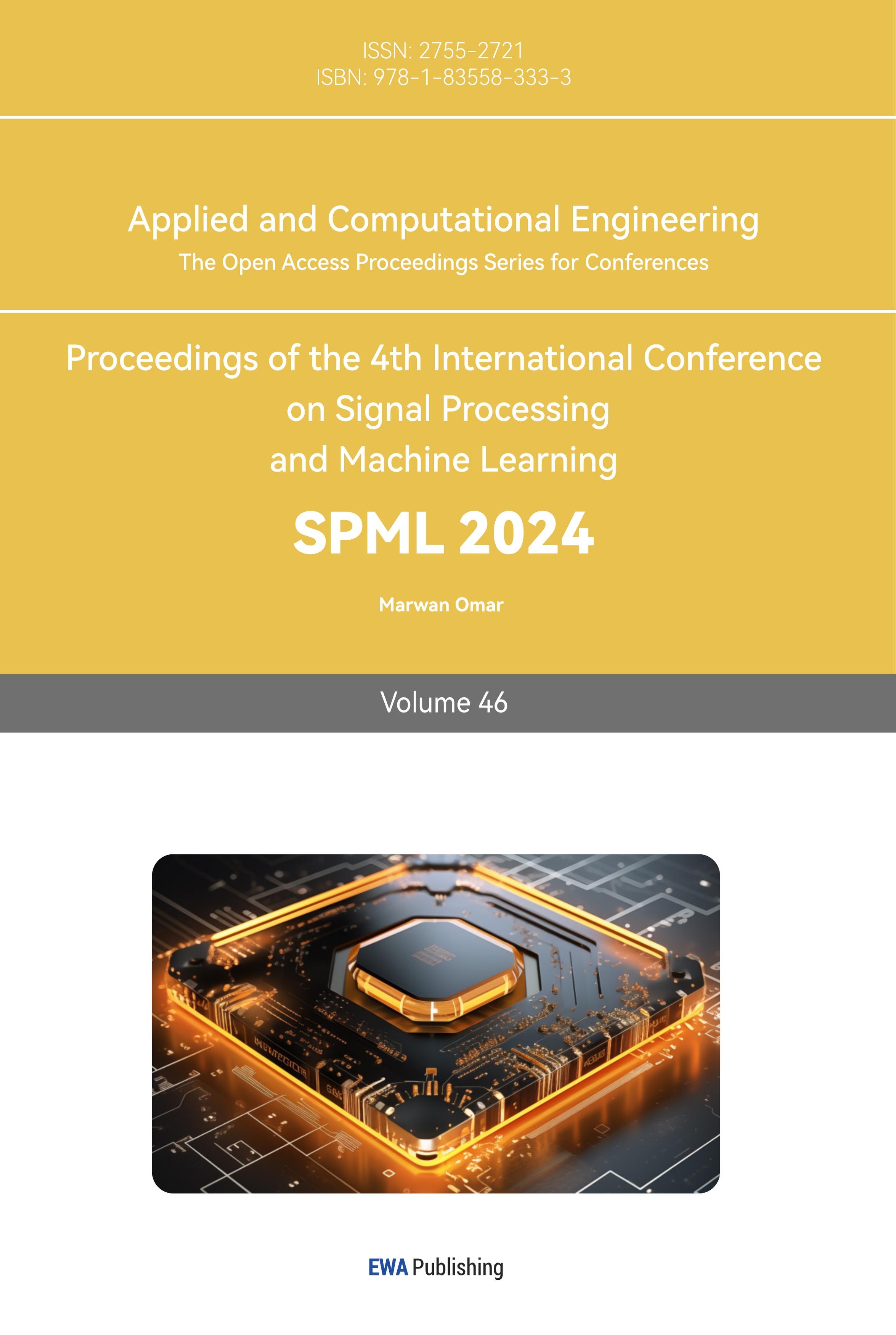
Conventional wheel models generally only have the ability to move in a single direction. One type of mobile robot chassis is the two-wheel differential drive chassis. Figure 1 shows a robot uses this chassis. The drive wheels are similar to conventional wheels, while the passive wheel is typically a ball caster or an omnidirectional wheel. To achieve lateral movement, this robot chassis relies on differential speed control of the drive wheels to change its direction while moving forward or backward. It is not a holonomic or omnidirectional wheel chassis, and it has a differential degree of freedom of 2 [1].

Another commonly used mobile robot chassis is the Car-Like chassis. This type of chassis is still not a holonomic chassis, as its kinematic characteristics restrict its lateral movement capability and ability to rotate in place [2].

Mecanum wheels changed robotic mobility by enabling omnidirectional movement through their unique wheel configuration. Mecanum wheels utilize rollers set at angles to provide lateral and diagonal motion, making them ideal for tight spaces.

In 1973, engineer Bengt Lion from the Swedish company Mecanum invented the Mecanum wheel and patented it under the company's name. The patent was purchased by the U.S. Navy in 1980 for military applications. After the expiration of the patent in 1996, it gained significant development and became a milestone for omnidirectional wheels. More and more companies have successfully applied it to their own developed equipment. For example, the youBot palletizing robot developed and manufactured by the German company KUKA is equipped with five degrees of freedom and a two-degree-of-freedom manipulator, enabling complex handling and assembly operations. The aircraft engine positioning device designed and applied by the German company MIAG allows wireless remote-controlled installation of equipment, even in confined spaces, enabling flexible transportation of aircraft components and improving installation efficiency [3].

The study of the kinematics and dynamics of mobile robots is the most fundamental research that reflects their maneuverability. It is also a core research area for implementing the lowest-level systems of mobile robots, providing a foundation for their applications. For wheeled omnidirectional mobile robots, the kinematic and dynamic models establish a relationship between the wheel output velocities or torques and the changes in the robot's chassis pose. Building on geometric mathematics, Gfrerrer·A analyzed the motion constraints of Mecanum wheels and provided calculation formulas for the characteristic parameters of roller mechanical design and processing [4]. This quantified the geometric structural properties of the rollers and addressed the procedural issues in Mecanum wheel mechanical design. Muir et al. established the kinematic model of the omnidirectional mobile robot platform "Uranus" using matrix transformation methods and applied this mathematical model to design robot feedback control algorithms and slip detection [5]. Campion et al. studied three-wheeled mobile robots, derived their kinematic models, and analyzed the motion characteristics of the robots under ideal constraint conditions based on the model [6]. Lin derived the kinematic and dynamic equations of Mecanum mobile robots under the typical conditions of uneven robot mass distribution and uncertain wheel-ground friction coefficients using Lagrange's equations [7]. Trajectory control of the robot was achieved through adaptive control methods.

2. Methords

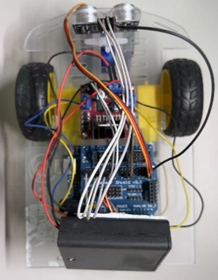
Robot coordinate transformation refers to two aspects: firstly, the transformation from the robot coordinate system to the world coordinate system, and secondly, the transformation from the world coordinate system to the robot coordinate system [8]. The former is used to map the actual motion of the robot in its own coordinate system to the world coordinate system, while the latter is used to map the desired motion in the world coordinate system to the robot coordinate system. Figure 2 shows the coordinates of the robot in the world coordinate system and the robot coordinate system.

To accomplish the coordinate system transformation, the rotation matrix of the robot about the Z-axis is required, as shown in Equation 1.

\( {R_{z}}=[\begin{matrix}cosθ & -sinθ & 0 \\ sinθ & cosθ & 0 \\ 0 & 0 & 1 \\ \end{matrix}] \) (1)

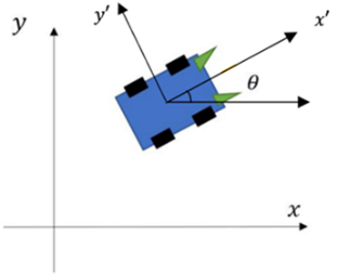
A Mecanum wheel is a commonly used omnidirectional wheel in mobile robots, which differs from regular rubber tires used in cars. As shown in Figure 3, the Mecanum wheel consists of a hub and rollers.

The labeled torque input in Figure 3 refers to the direct connection of the Mecanum wheel's hub to the output shaft of the robot chassis's motor. The rollers are connected diagonally at 45 degrees to the hub's bent bracket through bearings, but they are not directly connected to the motor. The rollers themselves are passive wheels mounted on the hub. Mecanum wheels are divided into left wheels and right wheels, as shown in Figure 4(a) and 4(b).

To analyze the characteristics of the Mecanum wheel's right wheel, it is important to focus on the frictional force vectors between the wheel and the ground. Therefore, the contact surface between the wheel and the ground should be taken as the reference point for analysis. The perspective top view of the Mecanum wheel's right wheel in contact with the ground is shown in Figure 5. Although it may appear similar to the Mecanum wheel's left wheel, its actual contact surface with the ground is opposite to that of the left wheel.

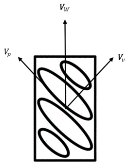
When viewed from the right side, as the right wheel of the Mecanum wheel rotates clockwise, the main wheel has a linear velocity \( {V_{w}} \) relative to the robot. Due to the free rolling of the rollers on the main wheel, as the robot moves, the rollers will decompose the velocity on the main wheel under the influence of the ground friction. This results in the Mecanum wheel experiencing rolling friction that does work only in the \( {V_{p}} \) direction, while in the \( {V_{v}} \) direction, the rollers will generate rotation and experience rolling friction with the ground that does no work. This portion of rolling friction is mostly absorbed by the bearings between the rollers and the hub. The relationship between \( {V_{p}} \) and \( {V_{w}} \) can be expressed as Equation 2.

\( {V_{P}}={V_{W}} ·cos{（45°） } \) (2)

In this case, the 45-degree angle represents the angle between the roller and the axis of the wheel hub, reflecting the decomposition effect of the roller on the velocity of the main wheel. Similarly, the Mecanum left wheel, which is symmetrical to the Mecanum right wheel, operates on similar principles. Its working direction is also symmetrical to that of the Mecanum right wheel.

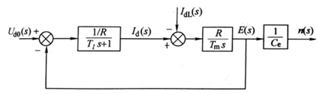
For dynamic modeling of the robot's motors, there is a modeling method by Martins F N based on motor characteristics, as represented by Equations 3, 4, and 5 [9].

\( n=\frac{{U_{d}}-{I_{d}}{R_{a}}}{{C_{e}}} \) (3)

\( {T_{e}}={C_{m}}{I_{d}} \) (4)

\( {T_{e}}-{T_{L}}=\frac{G{D^{2}}}{375}\frac{dn}{dt} \) (5)

If Equations 3, 4, and 5 are substituted and a Laplace transform is performed, the motor transfer function model is represented as shown in Figure 6. The parameters of the robot's wheel motor are as follows: Stall torque = 0.3 N*m; Stall current = 3 A; Rated voltage = 12 V; Rated current = 0.3 A; Armature resistance = 4 Ω; Rated speed = 550 rpm.

When analyzing the chassis, it is also important to consider the ground contact surface, which is the perspective top view of the robot chassis, as the reference point for analysis[10]. The motion of each wheel of the robot and the overall motion of the robot should be analyzed. Since the motion of a rigid body in a plane can be decomposed into three independent components: X-axis translation, Y-axis translation, and yaw rotation, a Cartesian coordinate system (XOY) is established based on the analysis in Figure 7. Based on the analysis, when the right rear wheel of the robot, namely the Mecanum left wheel, has a velocity \( {V_{w1}} \) relative to the robot, it generates an effective component velocity \( {V_{p1}} \) with a direction of 45 degrees relative to the ground and a magnitude of \( {V_{w1}}*cos{(45 °)} \) .

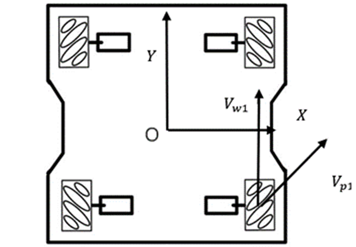
Based on Figure 7 and the previous analysis of individual wheel kinematics, the inverse kinematics model (Equation 6) and forward kinematics model (Equation 7) for a Mecanum wheel robot can be derived.

\( [ \begin{array}{c} {V_{1}} \\ {V_{2}} \\ {V_{3}} \\ {V_{4}} \end{array} ]=[\begin{matrix}1 & 1 & (a+b) \\ 1 & -1 & -(a+b) \\ 1 & 1 & -(a+b) \\ 1 & -1 & (a+b) \\ \end{matrix}][ \begin{array}{c} {V_{x}} \\ {V_{y}} \\ W \end{array} ] \) (6)

\( [ \begin{array}{c} {V_{x}} \\ {V_{y}} \\ W \end{array} ]=[\begin{matrix}-1 & 1 & -1 & 1 \\ 1 & 1 & 1 & 1 \\ \frac{1}{a+b} & \frac{-1}{a+b} & \frac{-1}{a+b} & \frac{1}{a+b} \\ \end{matrix}][ \begin{array}{c} {V_{1}} \\ {V_{2}} \\ {V_{3}} \\ {V_{4}} \end{array} ] \) (7)

For a four Mecanum wheel robot chassis, using the Lagrangian method to establish the dynamic model is a more convenient approach. This is because the Lagrangian method focuses on the system's kinetic and potential energies without the need to calculate internal forces. From the perspective of kinetic energy, the total kinetic energy of the robot includes the translational and rotational kinetic energies of the robot itself, along with the additional rotational kinetic energies of each wheel, as shown in Equation 8.

\( K=\frac{1}{2}m(v_{x}^{2}+v_{y}^{2})+\frac{1}{2}{I_{z}}{ω^{2}}+\frac{1}{2}{I_{w}}(ω_{1}^{2}+ω_{2}^{2}+ω_{3}^{2}+ω_{4}^{2}) \) (8)

In addition, due to the presence of ground friction that drives the acceleration of the vehicle body, the energy consumed by the rotation of each wheel when performing effective work is represented by F in Equation 9.

\( F=\frac{1}{2}{F_{ω}}(ω_{1}^{2}+ω_{2}^{2}+ω_{3}^{2}+ω_{4}^{2}) \) (9)

In Equation 8 and Equation 9, m represents the total mass of the robot, \( {I_{Z}} \) is the moment of inertia of the robot about the Z-axis, \( {I_{w}} \) is the moment of inertia of the wheels about the robot's center of rotation (also known as the centroid of the chassis), and \( {F_{ω}} \) is the coefficient of friction between the wheel sticks and the ground. Based on this, the conversion of the torques of the four motors of the robot chassis into Lagrange equations can be represented by Equation 10.

\( [ \begin{array}{c} {τ_{1}} \\ {τ_{2}} \\ {τ_{3}} \\ {τ_{4}} \end{array} ]=M[ \begin{array}{c} {\overset{¨}{q}_{1}} \\ {\overset{¨}{q}_{2}} \\ {\overset{¨}{q}_{3}} \\ {\overset{¨}{q}_{4}} \end{array} ]+λ[ \begin{array}{c} {\overset{˙}{q}_{1}} \\ {\overset{˙}{q}_{2}} \\ \overset{˙}{{q_{3}}} \\ {\overset{˙}{q}_{4}} \end{array} ] \) (10)

The matrices in Equation 10 are represented by Equations 11 to 15. The parameters of the robot chassis are as follows: Wheel radius = 0.5m; Wheelbase = 4m; Track width = 6m; Mass = 4kg; Robot's moment of inertia around the Z-axis = 2kg·m^2; Wheel's moment of inertia = 0.003kg·m^2.

\( M=[\begin{matrix}C & -D & D & F \\ -D & C & F & D \\ D & F & C & -D \\ F & D & -D & C \\ \end{matrix}] \) (11)

\( λ=[\begin{matrix}{λ_{1}} & 0 & 0 & 0 \\ 0 & {λ_{2}} & 0 & 0 \\ 0 & 0 & {λ_{3}} & 0 \\ 0 & 0 & 0 & {λ_{4}} \\ \end{matrix}] \) (12)

\( C=\frac{m{R^{2}}}{8}+\frac{{I_{z}}{R^{2}}}{16(L+1{)^{2}}}+{I_{w}} \) (13)

\( D=\frac{{I_{z}}{R^{2}}}{16(L+l{)^{2}}} \) (14)

\( F=\frac{m{R^{2}}}{8}-\frac{{I_{z}}{R^{2}}}{16(L+l{)^{2}}} \) (15)

According to the various research methods mentioned above, create a Simulink model and connect the signal lines appropriately. Then, add a Proportional Integral Derivative(PID) controller for the individual wheel speed loop and some peripheral components such as signal sources and scopes.

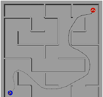
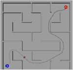
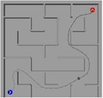
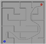
By connecting the Mecanum wheel robot model to the astar model in Robotics Playgrounds, the robot can follow the path generated by the A-star algorithm to test the applicability of the model, The maze is a 18m × 18m square maze. Setting the robot's start pose = [2 2 0]; goal pose = [16 16 pi/2], the A-star algorithm generates the path.

The results are shown in Figures 8(a), (b), (c), (d), and (e), which capture the robot's operation at 0s, 5s, 10s, 15s, 20s, and 20s, respectively. In Figure 8(a), (b), (c), (d), and (e), the blue dot represents the initial position of the robot, while the red dot represents the target position. The dark small dots represent the robot itself. The curve between the red and blue points in Figure 8(a), (b), (c), (d), and (e) represents the target path that the robot is tracking. It can be observed that the robot is able to track the trajectory.

3. Conclusions

By observing the results of the model's operation, it can be concluded that the model can achieve the goal of simulating the motion of a Mecanum wheel robot, including velocity signal tracking and path tracking. However, the model also has some limitations. Firstly, the battery voltage limitation in the robot dynamics section is a dynamic process in a real robot, mainly due to the internal resistance of the battery. Secondly, obtaining accurate robot parameters is challenging in practice. This model assumes certain parameters, but to accurately reflect the real-world scenario, parameters such as the robot's chassis moment of inertia and the wheel-ground friction coefficient need to be measured, which is not addressed in this research. Lastly, as the Mecanum wheel robot is a multi-in multi-out system, the Proportional Integral Derivative(PID) controller used in this model cannot linearize it and obtain theoretically optimal parameters. Instead, parameter tuning relies solely on empirical experience.

References

[1]. Malu S K, Majumdar J 2014 Kinematics, localization and control of differential drive mobile robot J. Global Journal of Research In Engineering pp 1-9.
[2]. De Luca A, Oriolo G, Samson C 2005 Feedback control of a nonholonomic car-like robot J. Robot motion planning and control pp 171-253.
[3]. Mohamed T B, Abd Karim N, Ibrahim N, Suleiman RFR, Idris MIB 2016 Development of mobile robot drive system using Mecanum wheels C. 2016 International Conference on Advances in Electrical, Electronic and Systems Engineering (ICAEES). IEEE pp 582-585.
[4]. Gfrerrer A 2008 Geometry and kinematics of the Mecanum wheel J. Computer Aided Geometric Design pp 784-791.
[5]. Muir P F, Neuman C P 1990 Kinematic modeling for feedback control of an omnidirectional wheeled mobile robot J. Autonomous robot vehicles pp 25-31.
[6]. Campion G, Bastin G, Dandrea-Novel B 1996 Structural properties and classification of kinematic and dynamic models of wheeled mobile robots J. IEEE transactions on robotics and automation pp 47-62.
[7]. Lin L C, Shih H Y 2013 Modeling and adaptive control of an omni-Mecanum-wheeled robot J.
[8]. Koditschek D E 1985 Robot kinematics and coordinate transformations C. 24th IEEE Conference on Decision and Control. IEEE pp 1-4.
[9]. Martins F N, Sarcinelli-Filho M, Carelli R 2017 A velocity-based dynamic model and its properties for differential drive mobile robots J. Journal of intelligent & robotic systems pp 277-292.
[10]. Hijikata M, Miyagusuku R, Ozaki 2023 Omni Wheel Arrangement Evaluation Method Using Velocity Moments J. Applied Sciences p13.
Cite this article
Sha,T. (2024). Mecanum wheels robot modeling and path tracking. Applied and Computational Engineering,46,246-253.
Data availability
The datasets used and/or analyzed during the current study will be available from the authors upon reasonable request.
Disclaimer/Publisher's Note
The statements, opinions and data contained in all publications are solely those of the individual author(s) and contributor(s) and not of EWA Publishing and/or the editor(s). EWA Publishing and/or the editor(s) disclaim responsibility for any injury to people or property resulting from any ideas, methods, instructions or products referred to in the content.
About volume
Volume title: Proceedings of the 4th International Conference on Signal Processing and Machine Learning
© 2024 by the author(s). Licensee EWA Publishing, Oxford, UK. This article is an open access article distributed under the terms and
conditions of the Creative Commons Attribution (CC BY) license. Authors who
publish this series agree to the following terms:
1. Authors retain copyright and grant the series right of first publication with the work simultaneously licensed under a Creative Commons
Attribution License that allows others to share the work with an acknowledgment of the work's authorship and initial publication in this
series.
2. Authors are able to enter into separate, additional contractual arrangements for the non-exclusive distribution of the series's published
version of the work (e.g., post it to an institutional repository or publish it in a book), with an acknowledgment of its initial
publication in this series.
3. Authors are permitted and encouraged to post their work online (e.g., in institutional repositories or on their website) prior to and
during the submission process, as it can lead to productive exchanges, as well as earlier and greater citation of published work (See
Open access policy for details).