1. Introduction

The stock market plays a pivotal role in shaping investment decisions, retirement planning, and the overall economic sentiment. Stock prices, thus, have always been at the center of attention for both retail and institutional investors. Predicting the ebb and flow of stock prices are of paramount interest to traders, investment banks, portfolio managers, and other market participants. Predicting stock prices also provides an opportunity for benchmarking, where the established model’s performance can be compared with other established models or results [1]. However, the dynamics of stock prices are influenced by many factors, some factors such as company-specific news are difficult to be evaluated. These factors introduce complexity to stock prices which makes the accurate prediction of stock prices a challenging task. Therefore, a high-fidelity model that predicts stock prices becomes indispensable and a high-fidelity model that predicts stock prices becomes indispensable.

A myriad of models and techniques have been employed over the decades to incorporate the multitude of factors affecting stock prices. Traditional approaches, such as statistic method like Autoregressive Integrated Moving Average (ARIMA) and simple machine learning methods like linear regression and logistic regression, offer simplicity and ease of interpretation but they both assume linear relation and it's sometimes difficult for them to capture complex long-term features [2]. On the other hand, more advanced deep learning model like GRU and LSTM harness the power of deep learning to recognize sequential patterns and long-term dependencies in stock price data [3]. And recently, an ensemble method primarily designed for structured data XGBoost have risen to prominence, given their ability to handle varied data types and offer robust predictive performance.

This paper focus on the stock price of two representative companies Google and Tesla. Google is a well-established tech giant with a long history in the stock market. Google's stock can be representative for developing models focused on stable, large-cap stocks and understanding how established companies' stock prices respond to industry-specific factors. While Tesla's stock can be representative for studying high-volatility stocks and exploring the impact of innovation, sentiment, and market dynamics on stock prices instead. Google's and Tesla's stock represent different facets of the stock market, high volatility and high variance in stock can add more challenges to predict accurately.

Two datasets are taken from Kaggle. Kaggle datasets often offer a level of standardization and are provided in a structured format suitable for analysis. This property offers benefit to this study since this study seeks to offer comparison of results between different models and datasets. A google stock price dataset and a Tesla stock dataset are chosen for this study. Both datasets contain 14 columns, where each column are assigned to an attribute and rows contains the values of that attribute. This study mainly focusses on 5 attributes: close, high, low, open, Volume. Such diverse datasets enable complex analyses, including multifactor prediction models [4].

The paper is organized as follows: In section 2, this paper introduces some relevant models that can be applied to stock price predicting area. In section 3, this paper shows the detail method of the models chosen, including data preprocessing, method explanation and model training methods. Section 4 presents the experimental findings, together with the corresponding comparison and interpretation of these data. In the next section, the conclusion of this study and the expected future works are presented. In the final section, all reference is listed.

2. Related works

Stock prices can be influenced by many different factors like company's financial situation, market sentiment and economic indicators. Stock price prediction and time series forecasting have been extensively researched areas with diverse methods being employed over the years. The methodologies encompass statistical approaches, machine learning techniques, deep learning methodologies, and a selection of hybrid methodologies.

The earliest proposed method to be applied in stock price prediction field is AutoRegressive Integrated Moving Average (ARIMA) which proposed in 1970s. ARIMA models can capture linear relationships in time series data, but those models assume constant variance over time which is not usually the case in stock prices [5]. Then Generalized AutoRegressive Conditional Heteroskedasticity (GARCH) models with the ability to change volatility over time were proposed in 1980s to overcome the limitation of ARIMA for handling non-constant variance property of stock prices [6]. The above two methods, however, assume statistic data and are still linear models at their cores.

To overcome the limitation of statistic data and linear model, RNN and their variant like LSTM networks and GRUs are designed to handle sequential data like stock prices. RNN faces the gradient vanishing and exploding problems and it's more sensitive to short term input which is not the case of stock price. LSTMs were introduced in 1990s over traditional RNNs since LSTMs have the ability to effectively capture long-term dependencies present in sequential data, while also addressing the issues of gradient disappearing and exploding. [7]. LSTMs address those by introducing a series of gate units to control the flow of information to be reminded or discarded. And with the ability to capture long-term dependencies, LSTMs can capture intricate patterns in stock price movements over extended periods.

Other traditional machine learning methods are also thought to be useful in the field of predicting stock prices. One of the most straightforward one, linear regression, has been extensively used for stock price prediction. Linear regression can establish a linear relationship between independent variables such as historical prices, but it also uses simple linear model and assumes constant variance of errors.

Moving beyond linear regression, decision trees partition the data space into regions and make predictions based on the mean response in each region. However, individual decision trees especially deep ones face the problem of overfitting and high variance, they can become too complex and becomes sensitive to noise. Until 2001, The purpose of Random Forest is to mitigate the danger of overfitting by combining the outcomes of numerous trees, it does well in providing insights into feature importance and capturing non-linear relationship with ensemble of trees structure. Then, Gradient Boosting Machines are proposed to handle sequential data like stock price by building trees sequentially. Also, each new trees of Gradient Boosting Machines would correct the errors of their predecessor, which allows them to provide more accurate results [8]. More recently in 2016, an implementation of Gradient Boosting Machines called Extreme Gradient Boosting (XGBoost) comes out and has now becomes one of the most popular and widely used implementations due to its amazing accuracy. XGBoost offers built-in regularization and built-in cross-validation which provides great efficiency and accuracy for develops [9].

Till now, more hybrid methods and deep learning methods like informers are being applied in the field of stock price prediction. In 2018, a hybrid deep learning method that combines CNN, RNN, LSTM was proposed. It makes use of the advantages of each model and is capable of capturing both short term and long-term features and gives accurate results. Informer is a model specifically designed to handle extreme long term sequential data. With self-attention mechanism, models like informers can focus on the more important time steps in the input stock price data and gives more nuanced prediction [10]. This paper integrates four main models mentioned above into the field of stock price predictions to evaluate how each model performs in this field.

3. Methodologies

In this study, since both chosen datasets have the same attributes, the data in both datasets is analyzed and preprocessed with exact same method. This study first downloads the row datasets from Kaggle and analyzes the row data using Pandas. Then this study preprocesses the row data to fit them into different models. the main models used in this study are Linear regression, RNN, LSTM networks, XGBoost. After the experiment of each model, an in-depth analysis of the comparison of result between different models is conducted.

3.1. Exploratory Data Analysis

This study analyzes an overview revealed the dataset’s attributes and data types, while a summary captured the statistical nuances of its numeric columns. To offer a temporal perspective, this study visualizes the (‘Open’, ’Close’, ’High’, ’Low’, ’Volume’) attributes of the datasets over time to better analyze the data features as shown in the dataset overview part of this paper.

3.2. Preprocessing

First, this paper normalizes the data using scikit-learn to rescale the data in a range of 0 to 1. Then, the data is divided into an 80% training set and a 20% testing set. in all the experiments to simulate real world unseen data. Also, this paper generates sequences and labels for training data and testing data as input to each specific model.

3.3. Model selection and construction

• SVR

SVR is a specialized variant of Support Vector Machines (SVM) that is specifically employed for regression problems. The objective is to identify a hyperplane in a high-dimensional space that optimally aligns with the given data, while adhering to a specified threshold.

The SVR model can be formulized as:

\( f(x)={w^{T}}x+b \) (1)

Where the weight matrix is denoted by \( w \) , the input feature vector is denoted as \( x \) , the bias term is denoted as \( b \) .

The goal of the SVR model is to minimize the following loss function:

\( L=\frac{1}{2}{||w||^{2}}+C\sum _{i=1}^{n}({ξ_{i}}+ξ_{i}^{*}) \) (2)

subject to

\( {y_{i}}-({w^{T}}{x_{i}}+b)≤ϵ+{ξ_{i}} \) (3)

\( ({w^{T}}{x_{i}}+b)-{y_{i}}≤ϵ+ξ_{i}^{*} \) (4)

\( {ξ_{i}},{ξ^{*}}≥0,i=1,2,…,N \) (5)

Where \( {ξ_{i}} \) and \( {ξ^{*}} \) are the slack variable, C is the regulation parameter, \( ϵ \) is the tube size, and n is the number of training samples. The parameter C balance between getting a flat plane and ensuring the data points within the tube.

• GRUs

GRUs stands out for addressing some limitations of traditional Recurrent Neural Network (RNN). Leveraging their effectiveness in mitigating the vanishing gradient problem, GRUs have gained significant popularity and are extensively employed across diverse domains within the field of machine learning. GRUs are computational efficient and easy to train with limit data with their simplified architecture with two gating mechanisms.

The working of GRU unit involves two gates: the update gate \( {(z_{t}}) \) and the reset gate \( ({r_{t}}) \) . Figure 1 gives a brief view into the detail structure of GRU unit. The following is the breakdown of the GRU unit:

Update gate ( \( {z_{t}} \) ): decides what fraction of the information of the previous hidden state ( \( {h_{t-1}} \) ) should be kept and what fraction of the new candidate state ( \( \widetilde{h} \) ) should be incorporated. The update gate can be computed by the formula below:

\( {z_{t}}=σ({W_{z}}[{h_{t-1}},{x_{t}}]) \) (6)

Where \( σ \) denoted the sigmoid activation function and \( {W_{z}} \) denoted weight matrices, \( {h_{t-1}} \) denoted the hidden state of last time step and \( {x_{t}} \) denoted the current input.

Reset gate ( \( {r_{t}} \) ): this gate determines what fraction of the previous hidden state should be forgotten and computes the new candidate state ( \( \widetilde{h} \) ). The reset gate can be computed by the formula below:

\( {r_{t}}=σ({W_{r}}[{h_{t-1}},{x_{t}}]) \) (7)

Candidate state ( \( \widetilde{h} \) ): A temporary memory that integrates information of \( {x_{t}} \) and \( {h_{t-1}} \) .

The candidate state can be formulized as follow:

\( \widetilde{{h_{t}}}=tanh{({W_{h}}[{r_{t}}{h_{t-1}},{x_{t}}])} \) (8)

Hidden state ( \( h \) ): The hidden state \( {h_{t}} \) is to store the integrated information of update gate \( {z_{t}} \) and the candidate state \( \widetilde{{h_{t}}} \) and the previous hidden state \( {h_{t-1}} \) , the update of hidden state can be formulized as follow:

\( {h_{t}}=(1-{z_{t}}){h_{t-1}}+{z_{t}}\widetilde{{h_{t}}} \) (9)

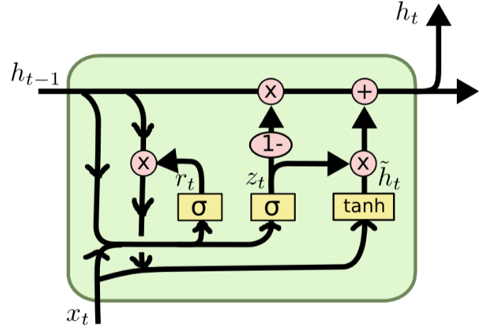
Figure 1. Structure of GRU units

In the context of our study, the input \( {x_{t}} \) is the sequence of the input features in the corresponding time step. GRUs are capable of capturing model sequential dependencies and capture patterns instead the sequences, which makes GRUs a useful tool for analyzing historical stock price data sequences.

• LSTM network

LSTM units are a type of RNN architecture. RNN faces the gradient vanishing and exploding problems and it's more sensitive to short term input which is not the case of stock price. And compared to GRUs, LSTM has a more complex architecture and has more controls over information flows. LSTMs are specifically designed to handle long-term dependencies, which means they can capture and remember patterns over long sequences more effectively than traditional RNNs. Given the sequential nature of stock prices, LSTMs can be especially useful in predicting stock market movements.

LSTMs address those by introducing a series of gate units to control the flow of information to be reminded or discarded [7]. Here, we introduce the basic principle of LSTM cells. Figure 2 shows the basic structure of LSTM units.

Here's a breakdown of the main components, Figure 2 shows the LSTM unit structure:

Forget Gate ( \( f \) ): The determination of what fraction of information of the cell state should be discarded or retained is made.

\( {f_{t}}=σ({W_{f}}[{h_{t-1}},{x_{t}}]+{b_{f}}) \) (10)

Input Gate ( \( i \) ): Determines the data that should be retained within the cell state.

\( {i_{t}}=σ({W_{i}}[{h_{t-1}}, {x_{t}}]+{b_{i}}) \) (11)

Cell State Update ( \( \widetilde{C} \) ): A candidate vector that has the potential to be incorporated into the cell state is undertaken.

\( {\widetilde{C}_{t}}=tanh{({W_{c}}[{h_{t-1}}, {x_{t}}]+{b_{c}})} \) (12)

New Cell State (C): The integration of information of the forget gate \( f \) , input gate \( i \) , and cell state update \( \widetilde{C} \) which results in the generation of a novel cell state.

\( {C_{t}}={f_{t}}×{C_{t-1}}+{i_{t}}×{\widetilde{C}_{t}} \) (13)

Output Gate (o): The determination of which component of the cell state is selected for output is made.

\( {o_{t}}=σ({W_{o}}[{h_{t-1}}, {x_{t}}]+{b_{o}}) \) (14)

\( {h_{t}}={o_{t}}×tanh{({C_{t}})} \) (15)

where \( σ \) is the sigmoid activation function, \( [{h_{t-1}},{x_{t}}] \) concatenates the previous hidden state and the current input. \( W \) and b represent weight matrices and bias vectors for each gate, respectively. \( {C_{t}} \) represent the cell state of each LSTM cell unit.

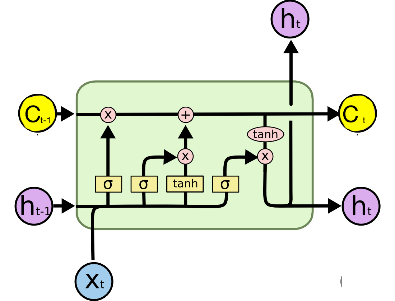
Figure 2. Structure of LSTM unit

Similar to GRU, a fix size slide window is used to slide through the input data to get the input sequences. LSTM performs excellent in handling long-term dependencies in sequential data, which is useful in this study.

• XGBoost

XGBoost, also known as Extreme Gradient Boosting, represents a sophisticated version of Gradient Boosting Machines. XGBoost is a very potent and adaptable machine learning algorithm renowned for its extraordinary efficacy in a diverse array of predictive modeling endeavors. The key feature of XGBoost includes gradient boosting, regularization, tree pruning and parallel processing which make use of modern computing resources (GPU).

The basic principle of Boosting is to integrate the results of weak models to generate a powerful composite model. Given a dataset \( D=({x_{1}},{y_{1}}),({x_{2}},{y_{2}}),…,({x_{m}},{y_{m}}) \) , where \( {x_{i}}={({x_{i,1}},{x_{i,2}},…,{x_{i,d}})^{T}} \) , \( {y_{i}}∈R \) . In this study, \( {x_{i,1}},{x_{i,2}},…,{x_{i,d}} \) represent the features such as historical volume of the stock, \( {y_{i}} \) represents the close value that need to be predicted. A tree ensemble method makes use of additive functions to forecast.

\( \hat{{y_{i }}}=ϕ({x_{i}})=\sum _{k=1}^{k}{f_{k}}({x_{i}}), {f_{k}}∈F \) (16)

Where \( F \) is the space of regression trees.

Here’s the formula of the built-in regularization of XGBoost:

\( L(ψ)= \sum _{i}l({\hat{y}_{i}}, {y_{i}})+\sum _{k}Ω({f_{k}}) \) (17)

Where \( l \) is the differentiable loss function, \( Ω \) is the model complexity.

The objective function of XGBoost measures both the model error \( L \) and the structural error \( Ω \) . The structural error of the model, represented by a regularization term, which is employed to constrain the complexity of the model. The model error measures the difference between the predicted sample value and the actual sample value. The following is the formula:

\( Obj(θ)=L(θ)+Ω(θ)=L({y_{i}},y_{i}^{t})+\sum _{k=1}^{t}Ω({f_{k}}({x_{i}})) \) (18)

3.4. Evaluation Metrics

This study utilizes various evaluation measures to assess the performance of the models, each of the metrics provide insight into the accuracy and variation of the predicted results.

• Mean Absolute Error (MAE)

MAE measures performance of a regression model, it’s the average magnitude of the errors between the true sample value and the predicted ones. MAE is commonly used in various domains including finance for predicting stock prices. MAE can be described by the following formula:

\( MAE=\frac{1}{n}\sum _{i=1}^{n}|{y_{i}}-\hat{{y_{i}}}| \) (19)

Where \( {y_{i}} \) is the predicted value and \( \hat{{y_{i}}} \) is actual value.

• Mean Absolute Percentage Error (MAPE)

MAPE measures the accuracy of the predicted results in terms of percentage errors. It’s a commonly used metric in forecasting tasks. MAPE can be described by the following formula:

\( MAPE=\frac{1}{n}+\sum _{i=1}^{n}|\frac{{P_{i}}-{A_{i}}}{{A_{i}}}|×100\% \) (20)

Where \( {P_{i}} \) is the predicted values and \( {A_{i}} \) is the actual values.

• Root Mean Squared Error (RMSE)

RMSE is more sensitive to outliers than MSE as it squares the error before averaging them. RMSE can also be useful when measuring the accuracy of the models. RMSE can be given by:

\( MSE=\frac{1}{n}\sum _{i=1}^{n}{({P_{i}}-{A_{i}})^{2}} \) (21)

The meaning of \( {P_{i}} \) and \( {A_{i}} \) remains the same as MAPE.

• R-squared ()

\( {R^{2}} \) measures how good do the model fits the data. It’s a statistical metric used to quantify the proportion of the variance seen in the dependent variable that can be explained or predicted by the independent variables. It computes how much of the variance in the dependent variable \( {P_{i}} \) is explained by the independent variable \( {A_{i}} \) :

\( {R^{2}}=1-\frac{\sum ({y_{i}}-\hat{{y_{i}}})}{\sum ({y_{i}}-\bar{y})} \) (22)

Where \( \bar{y} \) is the mean of the actual values of \( y \) .

4. Experimental setup and results

4.1. Dataset Overview

Table 1 shows the corresponding meanings of each attribute in both datasets. Figure 3 and Figure 4 shows the visualization of the four main attributes that we would focus on of GOOGLE and Tesla stock price dataset separately. Also, this study prints a heatmap to study the correlation between different features as shown in Figure 5, clearly, this is a highly correlated dataset. Figure 6 also presents the heatmap for the Tesla dataset, which shows similar feature with the heatmap for Google dataset.

Table 1. Description of the datasets

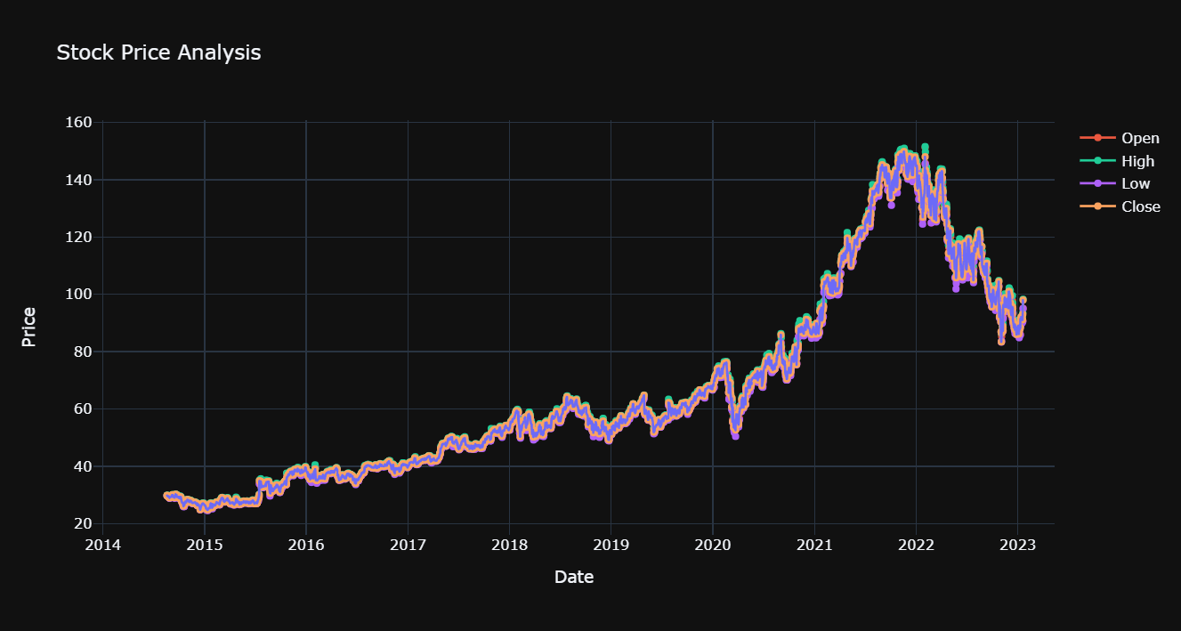
Figure 3. Visualization of Open High Low Close attributes of GOOGLE stock price.

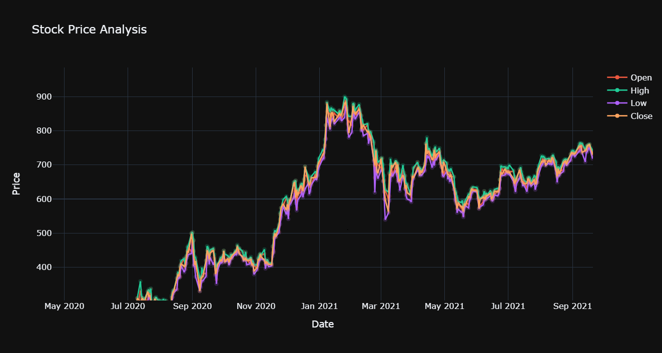
Figure 4. Visualization of Open High Low Close attributes of Tesla stock price.

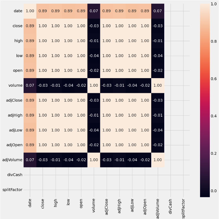
Figure 5. Heatmap of the google stock price.

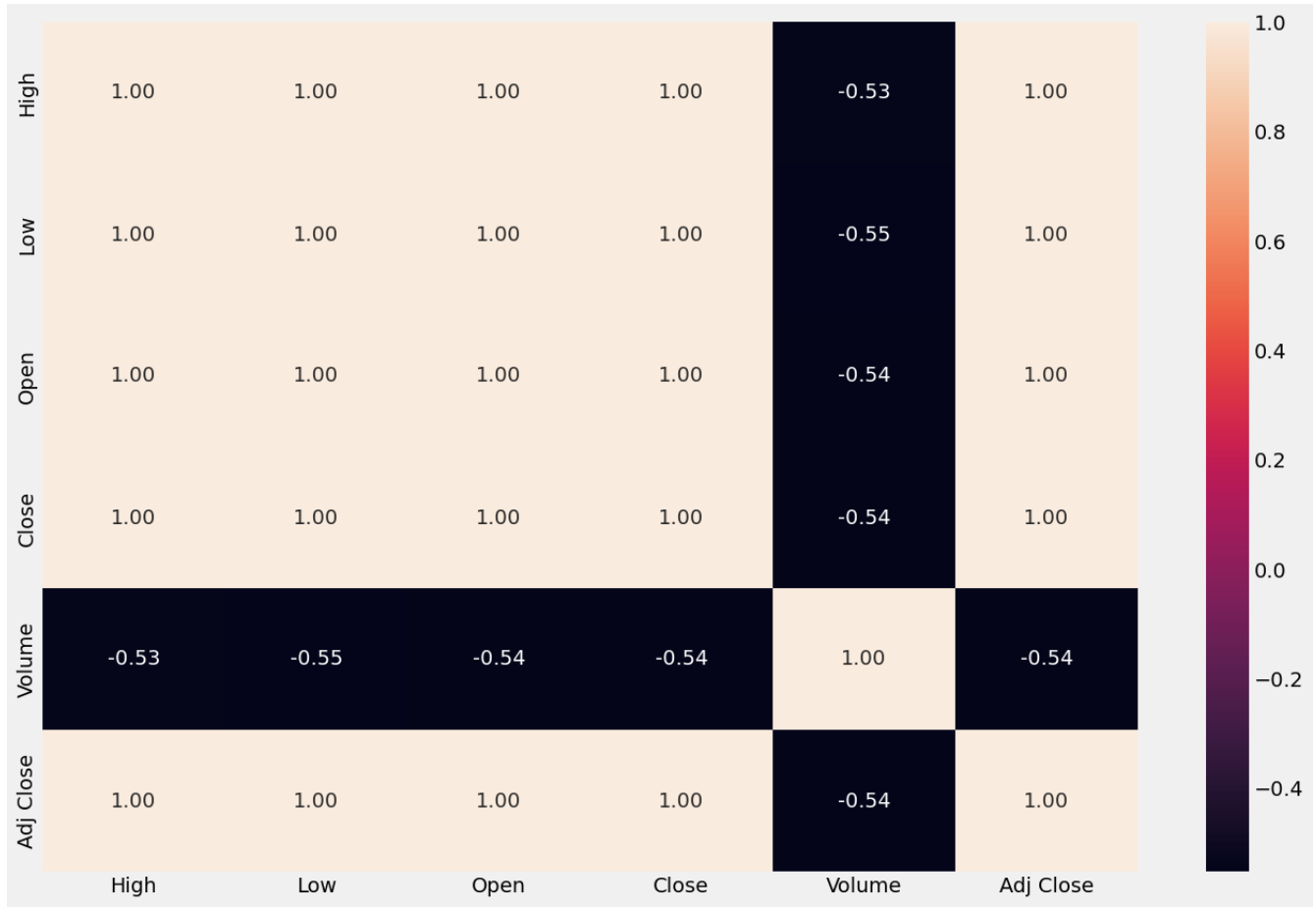
Figure 6. Heatmap of the Tesla stock price

4.2. Experimental Settings

The specific model architecture for each model is as follows:

• Linear regression

Single linear regression layer is utilized, with simple feature engineering that filters the volume attribute.

• Gate Recurrent Units

The data is reorganized into sequences of 20 time-steps after normalization. The activation function in each GRU layer is set to be tanh (Figure 7). This study trains the GRU model with batch size of 32 and 20 epochs. The optimizer is Adam, the loss is evaluated by mean squared error, and the evaluation metric is accuracy in keras.

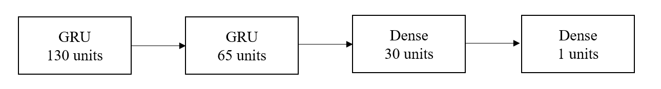
Figure 7. Structure of the GRU model

• Long Short-Term Memory network

The data features are reorganized into sequences of 40 time-steps after normalization. The model this study creates for stock price predictions is composed of three layers. The initial layer is a LSTM layer comprising 40 units, the input shape for this layer is defined as (40,5). Following this, the subsequent layer is also an LSTM layer, but with 50 units. Lastly, the last layer is a fully connected layer consisting of 5 units (Figure 8). The model is trained using a batch size of 16 and for a total of 250 epochs. The optimizer utilized in this study is Adam, while the chosen loss function is mean squared error. The evaluation metric employed to assess the model's performance is mean absolute error.

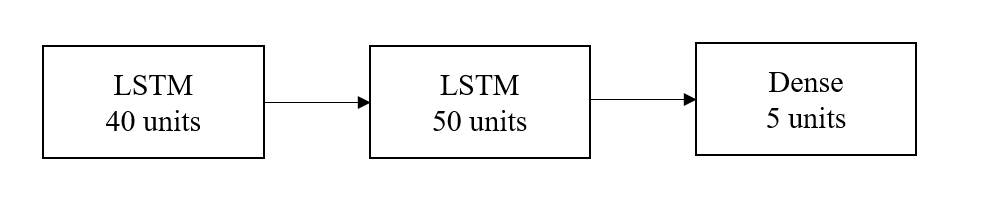
Figure 8. Structure of the LSTM model

• XGBoost

Two extra features: the difference between ‘High’ and ‘Low’ named ‘range_hl’ and the difference between ‘Open’ and ‘Close’ named ‘range_oc’ are added and used for model training. Moving average and standard deviation is calculated over a window size of 3, which helps to capture the trend and variability of the data. After hyper parameters tuning using Grid Search Cross-validation (CV), the best performed hyper parameters are determined. The max_depth is set to 8, min_child_weight is set to 2, while the learning rate is 0.1 and gamma is 0. Then the tuned model is trained using scaled training date.

4.3. Model Evaluation

The models are evaluated using RMSE, MAPE, R2 metrics on testing data. The evaluation results of the models on GOOGLE dataset are shown in Table 2. The results of evaluating the models on Tesla dataset are shown in Table 3.

Table 2. Evaluation of different models on GOOGLE stock price dataset.

Table 3. Evaluation of different models on Tesla stock price dataset.

5. Conclusion

In summary, this paper applies different machine learning models and deep learning models and time series models to find out the best method to predict stock prices. The model used includes SVR, GRU, LSTM and XGBoost. Each of these models are trained and evaluated using two different datasets. Among these models, LSTM is the best performing model in both datasets, for google stock price dataset: the RMSE is 0.00746, the MAPE is 1.49322, the R2 is 0.99650, the MAE is 0.00559, for Tesla stock price dataset: the RMSE is 0.00557, the MAPE is 0.97999, the R2 is 0.99526 and the MAE is 0.00395. LSTM performs well in every evaluation metric since LSTMs can storing long term information and capture feature patterns in time sequence data. Apart from LSTM, XGBoost also performs relatively well in capturing the important features and predicting stock prices. With more complex features engineering exists, XGBoost would perform even better and XGBoost can also measure the importance of each feature. Apart from this, hybrid models are also effective for stock price predictions. LSTM-CNN makes use of both LSTM’s strength in modeling sequential data and CNN’s capture spatial patterns, make it particularly suitable to fit time-series data.

References

[1]. Bao, W., Yue, J., & Rao, Y. (2017). A deep learning framework for financial time series using stacked autoencoders and long-short term memory. PloS one, 12(7), e0180944.
[2]. Tsay, R. S. (2010). Analysis of financial time series. _John Wiley & Sons_.
[3]. Hochreiter, S., & Schmidhuber, J. (1997). Long short-term memory. _Neural computation_, 9(8), 1735-1780.
[4]. Wang, Y. (2019). Stock price prediction using LSTM, RNN and CNN-sliding window model. arXiv preprint arXiv:1909.12207.
[5]. Box, G. E., & Jenkins, G. M. (1970). Time series analysis: forecasting and control. San Francisco: Holden-Day.
[6]. Engle, R. F. (1982). Autoregressive conditional heteroscedasticity with estimates of the variance of United Kingdom inflation. Econometrica: Journal of the Econometric Society.
[7]. S. Hochreiter and J. Schmidhuber, "Long Short-Term Memory," in Neural Computation, vol. 9, no. 8, pp. 1735-1780, 15 Nov. 1997, doi: 10.1162/neco.1997.9.8.1735.
[8]. Friedman, J. H. (2001). Greedy function approximation: a gradient boosting machine.
[9]. Chen, T., & Guestrin, C. (2016). XGBoost: A Scalable Tree Boosting System. In Proceedings of the 22nd ACM SIGKDD International Conference on Knowledge Discovery and Data Mining (pp. 785-794).
[10]. Zhou, S., Chen, J., Wang, J., Wen, C., Wang, Y., & Wu, Y. (2021). Informer: Beyond Efficient Transformer for Long Sequence Time-Series Forecasting.
Cite this article
Ye,S. (2024). Applying ensemble learning to multiple stock price predictions: A comparative study. Applied and Computational Engineering,50,189-198.
Data availability
The datasets used and/or analyzed during the current study will be available from the authors upon reasonable request.
Disclaimer/Publisher's Note
The statements, opinions and data contained in all publications are solely those of the individual author(s) and contributor(s) and not of EWA Publishing and/or the editor(s). EWA Publishing and/or the editor(s) disclaim responsibility for any injury to people or property resulting from any ideas, methods, instructions or products referred to in the content.
About volume
Volume title: Proceedings of the 4th International Conference on Signal Processing and Machine Learning
© 2024 by the author(s). Licensee EWA Publishing, Oxford, UK. This article is an open access article distributed under the terms and
conditions of the Creative Commons Attribution (CC BY) license. Authors who
publish this series agree to the following terms:
1. Authors retain copyright and grant the series right of first publication with the work simultaneously licensed under a Creative Commons
Attribution License that allows others to share the work with an acknowledgment of the work's authorship and initial publication in this
series.
2. Authors are able to enter into separate, additional contractual arrangements for the non-exclusive distribution of the series's published
version of the work (e.g., post it to an institutional repository or publish it in a book), with an acknowledgment of its initial
publication in this series.
3. Authors are permitted and encouraged to post their work online (e.g., in institutional repositories or on their website) prior to and
during the submission process, as it can lead to productive exchanges, as well as earlier and greater citation of published work (See
Open access policy for details).