1. Introduction

Due to the development and application of computer technology, mobile robots are widely used in today's production fields, especially in warehousing and logistics. For the design and development of mobile robots, path planning is crucial because it is necessary to reach a set destination from a known starting point while satisfying certain conditions. In real-world environments, it is crucial for mobile robots to accomplish tasks through path planning, e.g., mobile robots avoiding obstacles in dynamic fields, self-driving vehicles, or drones [1-3]. Common path planning algorithms fall into three categories based on various sampling techniques. Dijkstra algorithm [4], A* algorithm [5], and other graph-based search algorithms are examples. Planning techniques based on sampling include the RRT algorithm [6], the RRT* algorithm [7], and so on. Ant colony algorithm, genetic algorithm, and other heuristic-based planning algorithms are examples. Among them, for example, heuristic information is used by the A * algorithm, a heuristic algorithm, to choose the best course of action.Its disadvantages include low real-time performance, large computational complexity, and lengthy computation times for each node. Additionally, the algorithm's search efficiency declines with the number of nodes. Furthermore, not every possible solution is explored by the A * algorithm, and the outcomes might not always be the best option. So this article chose the RRT algorithm to improve the accuracy and reliability of path search as much as possible.

Lavalle introduced the RRT method in 1998.By choosing sampling locations at random inside the sampling area of the RRT algorithm, one can plan the route from the start point to the destination point. Because the RRT algorithm is probabilistic, it can determine the path if there is a viable path in the surroundings and there is sufficient time available. But the route that it chooses isn't always the best one.By reselecting the parent node and pruning, the RRT* algorithm was developed to shorten the generated path [8]. RRT * also has some drawbacks, such as blind node expansion and slow convergence rate. The reselection of the parent node has significant randomness and cannot quickly achieve the optimal result.

RRT * performs parent node comparison on the basis of RRT, ensuring that the parent node closest to the root node within the specified range is selected. At the same time, the algorithm also adds path optimization, which does not stop traversing after finding a feasible path for the first time, but does not stop until the specified number of iterations. During this process, as long as there is a new feasible path and the distance is shorter than the previous feasible path, the path is updated. Theoretically, the path obtained by the algorithm is Asymptotically optimal algorithm. If the number of iterations is unlimited, the path obtained will be infinitely close to the optimal path. Karaman et al. proposed the RRT* algorithm with progressive optimization, which effectively improves the searched path quality by reselecting the parent node and rewiring it in the exploration process.[9]

This article uses the most basic control variable method to control several basic variables in the RRT algorithm. And through multiple experiments, different experimental images and times were obtained to compare the advantages and disadvantages of the path and the amount of time. Among them, research is conducted on variables such as node number, step size, and observer number one by one, striving to find the most reasonable parameters to obtain the optimal path planning. The research results of this paper can be used to build the model of autonomous vehicle path planning. By limiting some variables, the computational complexity is reduced, making it easier to find the optimal path planning.

2. Related work

2.1. RRT Algorithm

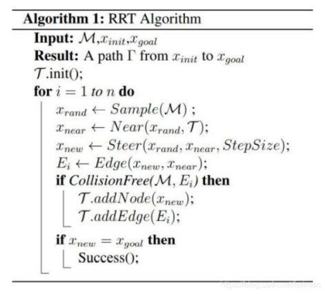
Figure 1. The principle of RRT algorithm

First, the algorithm produces random points to create a space-filling tree. Then, the enlargement of the random sample point expands to a gigantic unsearched area in order to find the path. Therefore, RRT can handle complicated and in-deterministic spaces with random obstacles, high-dimension and dynamic spaces, like reality.[10]

2.2. Programming

This article will implement the RRT algorithm in MATLAB and complete the construction of a visual model. And optimize the constructed model by changing multiple variables separately. Fully experiment and understand the characteristics of the RRT algorithm. Timing each debugging run also helps provide performance feedback. The acquisition of each time is based on the average of three repeated experiments. During the process of running the RRT algorithm, built-in parameters should also be changed to observe changes in performance time and search accuracy. After running the RRT algorithm, you should also compile the RRT * algorithm, optimize it from a theoretical perspective, and check the differences between the two.

In the process of programming in MATLAB, it is mainly divided into the following blocks: 1. Define the starting and ending points of obstacles; 2. Define RRT parameters (node number and step size); 3. Initialize and construct RRT; 4. Find the nearest node; 5. Expand and draw the tree; 6. Traverse back to the starting point from the endpoint, construct the path; 7. Draw the path; 8. Collision detection function and drawing function.

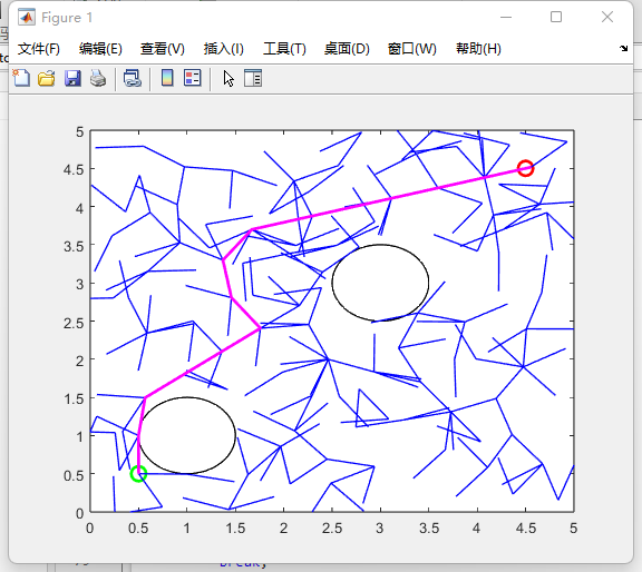
During code debugging, timing can be performed to visually view performance differences. This article will study the performance of the RRT algorithm by changing conditions such as the number of nodes, step size, and number of objects. The performance here includes runtime and path accuracy. Finally, the RRT * algorithm will be used to further optimize the entire program and display the results. In the visualization model below, the green dot is the starting point, the red dot is the ending point, the pink line is the path, and the blue line is the path branch. The original number of nodes is 500, and the original step size is 0.5.

3. Methods

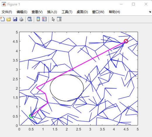
This article uses code for simulation under basic parameters. The node number is 500, the step size is 0.5, the starting point is (0.5, 0.5), and the focus is (4.5, 4.5). Obstacles are two circles with a radius of 0.5 at the centers of (1, 1) and (3, 3).

Figure 2-11 shows the final result of the simulation and the steps of the algorithm using MATLAB. The green dots are the starting points, the red dots are the end points, the pink lines are the paths after this simulation, and the blue lines are the branches in the search process. In addition, the horizontal and vertical coordinates in the icons are the location parameters, respectively.

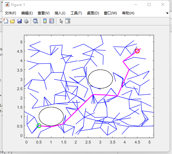
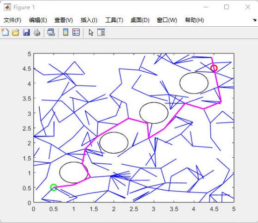
Fig. 2 shows the original process of a complete path search. In this case, the paths appear to be extremely cluttered, and the blue lines in Figure 2 are cluttered and disorganized. Secondly, the number of nodes is adjusted based on the original process, and the result is shown in Figure 3 without affecting the changes in other values. Doubling the number of nodes and holding other variables constant increases the search time considerably, but the path accuracy is not significantly improved. The overall change does not differ much from Figure 2. In addition, the step size was adjusted. The authors chose to reduce the step size to 0.1, and with other variables unchanged, the results are shown in Figure 4. The accuracy of the path is improved relative to Figure 3.

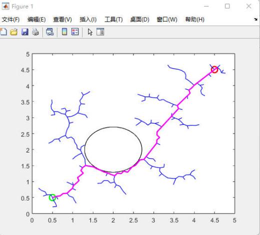
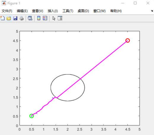
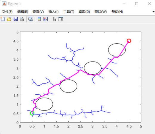
Figure. 5 shows the insignificant change in the accuracy of the path in the case where the obstacles are merged as linked obstacles but with the same area and other variables are kept constant. Therefore, the authors have reduced the step size to 0.1 based on Figure 5, with linked obstacles and ensuring the same area while keeping other variables constant. The result is shown in Figure 6. Based on the change in the above pairs, the authors further adjusted the step size by reducing the step size to 0.01, linked obstacles to the same area while keeping all other variables unchanged. The results are shown in Figure 7 with improved accuracy.

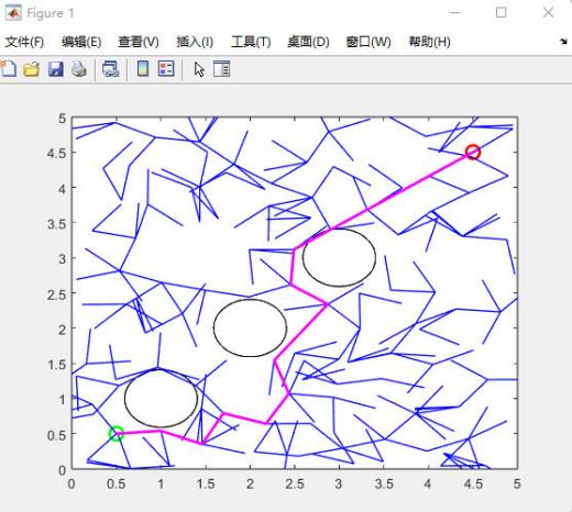
The experiment was then further upgraded by increasing the number of obstacles to 3 and ensuring that each obstacle had the same area. When the number of obstacles was adjusted and all other conditions remained the same, the accuracy of the paths did not change much (Figure 8).

Following this, the authors chose to continue adding obstacles, increasing the number of obstacles to 4 and ensuring that the obstacles had the same area. Figure 9 shows a plot of the simulation results when the number of obstacles is 4 (each with the same area) with no change in their conditions and no significant change in the accuracy of the path. Based on Figure 9, the step size was further adjusted and reduced to 0.1 to produce Figure 10, which shows the simulation results when the number of obstacles is increased to 4 and each obstacle has the same area, and the step size is reduced to 0.1, with no change in the other conditions. According to the picture, it can be seen that the accuracy of the path is improved compared to Figure 9.

In figure 11, it shows the situation when uses RRT* algorithm to optimize the program.The pink and light blue lines are the final paths, and it can be seen that both paths are quite close to the optimal path.

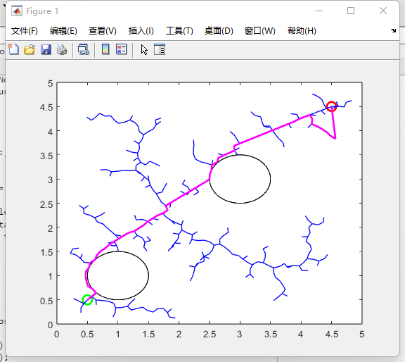
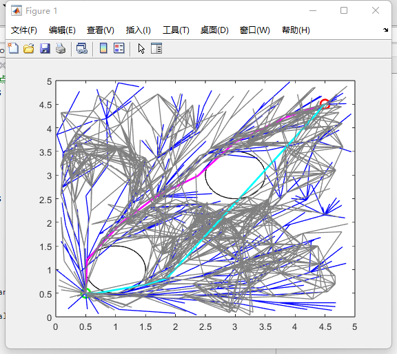
This table displays the average running time after three tests under different conditions. It can be seen that in the figure of number 5, the average time is the lowest at 90s. However, in figure 11, the average time is 1028s, which is almost 11 times than the former one.

Table 1. Time Table

4. Result

When using the RRT algorithm for path planning, there are many situations that can occur due to excessive randomness. However, based on the experimental results mentioned above, it can be seen that the factors affecting the results include setting the number of nodes, modifying the step size, and setting obstacles. Among them, the setting of the number of nodes has a great impact on the running speed, but it does not necessarily provide a more accurate path. Modifying the step length also optimizes the running time, but at the same time produces a limited final result. In addition, according to the runtime comparison in Table 1, the setting of obstacles on the map also has an impact on the program's runtime speed.

In general, reducing the step size can indeed improve the search accuracy, regardless of whether the obstacles are connected or split. With respect to the modeling experiments established in this paper, it can be seen that the path accuracy is higher when the step size is 0.1. Too small a step can actually lead to the inability to complete a complete path search.

The RRT * algorithm can theoretically be used to optimize the entire path search process. Specifically, the RRT * algorithm will reconnect the shorter path between the new node and its parent node based on the original RRT algorithm to obtain a better path. However, it also takes a relatively longer time. This also shows that the RRT* algorithm needs more optimization and adjustment in practical applications. However, the current experimental findings can also be applied to the field of autonomous driving to allow vehicles to find better paths in a shorter time.

5. Conclusion

This article investigates many basic parameters of the RRT algorithm in path planning. We used the MATLAB platform for simulation experiments, using the most basic control variable method and the method of averaging multiple experiments to avoid randomness. Firstly, divide the RRT algorithm into multiple parts and complete the entire program writing work. Then start changing the various variables in the algorithm, and observe the time of the final path and measure the running time. This includes variables such as number of nodes, step size, and obstacles. Among them, step size has a significant impact on the accuracy of the generated path. The conclusion drawn in this article is that finding the appropriate step size can greatly improve the accuracy of path planning. Of course, the RRT algorithm is not perfect and can also be optimized using the RRT * algorithm, but this requires multiple times to improve the accuracy of the path. This indicates that the RRT * algorithm still needs more optimization. These conclusions can be applied to the field of autonomous driving, allowing vehicles to find better paths in a shorter time.

However, this article also has certain limitations. The application improvement of RRT algorithm can only stay at the qualitative level, and cannot build an adaptive learning machine model. The continuous optimization of various parameters in the RRT algorithm based on artificial intelligence machine models is the direction that this article can optimize. The research on RRT * algorithm is not very sufficient, and in-depth research on this advanced algorithm is also the optimization direction of this article. Finally, due to the high randomness of the RRT algorithm, the various legends presented in this article may not represent a common situation and may have some chance. In the future, the advantages and disadvantages of the path can be visualized by measuring the length of the path. The obstacles used in this article are relatively simple, only a few circular obstacles, and there is no in-depth exploration of more complex obstacle situations. In the future, the performance of the RRT algorithm can also be tested by changing the shape of the obstacles, such as setting a maze.

References

[1]. B. K. Patle B. Babu L, A. Pandey, D. R. Parhi, and A. Jagadeesh, “A review: On path planning strategies for navigation of mobile robot,” Defence Technology, vol. 15, no. 4, pp. 582–606, 2019.
[2]. C. Badue, R. Guidolini, R. V. Carneiro, P. Azevedo, V. B. Cardoso, A. Forechi, L. Jesus, R. Berriel, T. M. Paixão, F. Mutz, L. de P> Veronese, T. Oliveira-Santos, and A. F. de Souza, “Self-driving cars: A survey,” Expert Systems with Applications, vol. 165, 2021.
[3]. S. Aggarwal and N. Kumar, “Path planning techniques for unmanned aerial vehicles: A review, solutions, and challenges,” Computer Communications, vol. 149, pp. 270–299, 2020.
[4]. Dijkstra, E. W. (1959). A note on two problems in connexion with graphs. Numerische mathematik, 1(1), 269-271.
[5]. Hart, P. E., Nilsson, N. J., & Raphael, B. (1968). A formal basis for the heuristic determination of minimum cost paths. IEEE transactions on Systems Science and Cybernetics, 4(2), 100-107.
[6]. LaValle, S. M. (1998). Rapidly-exploring random trees: A new tool for path planning.
[7]. Karaman, S., & Frazzoli, E. (2011). Sampling-based algorithms for optimal motion planning. The international journal of robotics research, 30(7), 846-894.
[8]. Benxue Liu & Chong Liu (2022). Path planning of mobile robots based on improved RRT algorithm.J. Phys.: Conf. Ser. 2216 012020
[9]. Xuewu W ,Jin G ,Xin Z , et al. Path Planning for the Gantry Welding Robot System Based on Improved RRT*[J]. Robotics and Computer-Integrated Manufacturing, 2024, 85.
[10]. Qianshi Z ,Minyu L ,Yizhe S . RRT path planning algorithm with enhanced sampling[J]. Journal of Physics: Conference Series, 2023, 2580(1).
Cite this article
Yao,J. (2024). RRT algorithm learning and optimization. Applied and Computational Engineering,53,296-302.
Data availability
The datasets used and/or analyzed during the current study will be available from the authors upon reasonable request.
Disclaimer/Publisher's Note
The statements, opinions and data contained in all publications are solely those of the individual author(s) and contributor(s) and not of EWA Publishing and/or the editor(s). EWA Publishing and/or the editor(s) disclaim responsibility for any injury to people or property resulting from any ideas, methods, instructions or products referred to in the content.
About volume
Volume title: Proceedings of the 4th International Conference on Signal Processing and Machine Learning
© 2024 by the author(s). Licensee EWA Publishing, Oxford, UK. This article is an open access article distributed under the terms and
conditions of the Creative Commons Attribution (CC BY) license. Authors who
publish this series agree to the following terms:
1. Authors retain copyright and grant the series right of first publication with the work simultaneously licensed under a Creative Commons
Attribution License that allows others to share the work with an acknowledgment of the work's authorship and initial publication in this
series.
2. Authors are able to enter into separate, additional contractual arrangements for the non-exclusive distribution of the series's published
version of the work (e.g., post it to an institutional repository or publish it in a book), with an acknowledgment of its initial
publication in this series.
3. Authors are permitted and encouraged to post their work online (e.g., in institutional repositories or on their website) prior to and
during the submission process, as it can lead to productive exchanges, as well as earlier and greater citation of published work (See
Open access policy for details).