


1. Introduction
Artificial Intelligence's Reinforcement Learning (RL) paradigm bears a striking resemblance to natural learning processes in humans and other animals, diverging notably from conventional Machine Learning (ML) methodologies. RL algorithms, often inspired by biological learning systems [1], eschew the reliance on pre-labeled data typical of Supervised Learning. Instead, RL agents learn through interaction, taking actions and receiving feedback from the environment without explicit instruction on each move [2]. This process involves an agent impacting its environment, observing the resultant changes, and receiving rewards or penalties, gradually evolving a strategy to optimize outcomes [3-6].
A pivotal challenge in RL is the Exploration and Exploitation (EE) dilemma. In this context, agents often favor actions known to yield high rewards (exploitation) to maximize cumulative gains [7,8]. However, such a strategy might trap agents in suboptimal choices, neglecting untried or incompletely explored actions that could offer superior rewards. Consequently, an agent must balance exploiting known actions with exploring new possibilities [9]. Central to RL research is the Multi-Armed Bandit (MAB) problem, embodying this balance between exploration and exploitation [10]. The MAB problem is a model of decision-making where the objective is to strike a balance between leveraging past successful actions and probing potentially more rewarding future actions. Facing a set of choices, the decision-maker selects one at each step, receiving an associated reward, the magnitude of which is unknown beforehand [11,12]. The aim is to maximize cumulative rewards over time, while minimizing the "regret" - the loss incurred by not choosing the optimal action.
MAB algorithms have found diverse applications, including in recommendation systems, clinical trials, and financial investment [11-13]. New models and approaches continue to emerge, expanding into areas like Contextual, Linear, and Combinatorial Bandits. This paper commences with an examination of classic MAB algorithms - Explore-Then-Commit, Epsilon-Greedy, SoftMax, Upper Confidence Bound, and Thompson Sampling. It delves into the factors influencing their performance, compares them with their variants, and discusses new models and applications in the MAB domain [14].
2. Relevant theories
2.1. Reinforcement learning model
Reinforcement Learning is a machine learning approach aimed at learning how to make decisions by interacting with an environment to maximize or minimize a specific objective function. Unlike supervised and unsupervised learning, reinforcement learning doesn't require labeled datasets or explicit answers; instead, it learns through trial and error by interacting with the environment [15]. As shown in figure 1.
In order to learn how to make the best decisions, a learning agent in reinforcement learning monitors the status of the environment, acts, and receives reward signals from it. Usually, Markov Decision Processes (MDPs) are used to formalize situations involving reinforcement learning. Key concepts in reinforcement learning include:
State: Describes a specific situation or condition of the environment. In a given state, the agent can take different actions [16].
Action: The possible choices or actions the agent can make in a given situation.
Reward: The environment's feedback signal, which indicates how excellent or poor the agent's action was, after it has been taken. Rewards may be zero, negative, or positive.
Policy: The way or rule by which the agent selects actions based on the current state. Policies can be deterministic (deterministic policy) or stochastic (random policy).
Value Function: Used to evaluate the long-term return for a specific state or state-action pair. Value functions help the agent determine which actions are better to take.
Environment Model: A model used to simulate the dynamics of the environment. Some reinforcement learning algorithms require an environment model for learning, while others directly interact with the real environment.
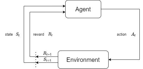
Figure 1. Reinforcement Learning Interaction Process (Photo/Picture credit: Original).
2.2. Stochastic multi-armed bandit problem
In reinforcement learning, the Stochastic Multi-Armed Bandit Problem is a common model that addresses the trade-off between exploration and exploitation [17-20]. The MAB problem is a sequential decision-making problem. This name originates from the slot machine in the casino. The gamer wants to get the highest reward by pulling different arms. Formally, there are \( k \) arms labeled with 1 to \( k \) . The \( ar{m_{i}} \) is related to an unknown distribution \( {F_{i}} \) and the expectation of the reward is \( {μ_{i}} \) . The agent will make decisions over \( n \) rounds called horizon. At each time step, the agent will choose an \( ar{m_{i}} \) and receive a reward \( {X_{t}} \) based on the distribution. If the agent knows which arm has the largest expectation of the reward in advance, it just needs to choose this arm each round. However, because the distribution \( {F_{i}} \) is unknown, the agent must balance exploration for finding the best arm and exploitation for choosing the current best arm to get the highest reward. The cumulative expected regret serves as a measurement for the MAB algorithm's performance, which for any fixed round \( n \) is defined as:
\( {R_{n}}=n\cdot {μ^{*}}-E[\sum _{t=1}^{n} {X_{t}}] \) (1)
where \( {μ^{*}}=max{{μ_{i}}}, i = 1,…,k \) , denotes the expected reward of the best arm.
3. Method
The paper focuses on the many bandit algorithms' processes as well as the examination and comparison of the various classic bandit algorithms' and their variants' performances across various horizons and parameters.
3.1. Classic Bandit Algorithms
3.1.1. Explore-Then-Commit. The Explore-Then-Commit is a classic bandit algorithm. To overcome the EE dilemma, the algorithm utilizes a relatively simple strategy just like the A/B test that divides the whole algorithm into two phases: the exploration phase and the exploitation phase. In the exploration phase, the algorithm will select each arm sequentially to explore each arm the same number of times and get the estimate of the average reward of each arm [21]. In the exploitation phase, the algorithm will only select the arm that has the highest estimate of the average reward so that the algorithm can make the cumulative regret as small as possible in this phase. The ETC policy is given in Table 1 below.
Table 1. ETC policy
Algorithm 1 Explore-Then-Commit Algorithm |
Input: \( m: \) Number of times each arm will be explored 1: for \( t = 1,2,3,…,T \) do 2: if \( t≤mk \) then 3: Choose \( ar{m_{i}} \) where \( i=(t mod k)+1 \) 4: Choose the reward \( {X_{t}} \) and update \( {\hat{μ}_{i}} \) 5: else 6: Choose \( ar{m_{i}} \) where \( i=argma{x_{i}}({\hat{μ}_{i}}) \) 7: end if 8: end for |
k stands for the number of arms. \( {\hat{μ}_{i}} \) embodies the average reward of \( ar{m_{i}} \) given in the exploration phase as an estimate of the real average reward of \( ar{m_{i}} \) .
The main feature of the ETC algorithm is shown in the pseudocode. The algorithm will explore each arm for \( m \) times and then immediately start the exploitation phase [22]. Though this policy is easy to understand and implement, the transition from exploration to exploitation is too abrupt. To balance the exploration and exploitation more reasonably, the following algorithms are introduced.
3.1.2. SoftMax. The SoftMax algorithm refers to the Boltzmann distribution in the physics field so the SoftMax is also called the Boltzmann Exploration. To solve the EE dilemma, the algorithm determines which arm to choose in each round by first calculating a weight or probability for each arm, and then selecting the arm whose probability is the highest. The probability for the algorithm to select an arm follows the following formula:
\( P(j)=\frac{{e^{{\hat{μ}_{j}}/τ}}}{\sum _{i=1}^{k} {e^{{\hat{μ}_{i}}/τ}}} \) \( \) (2)
In this formula, \( τ \) is a hyperparameter whose physical meaning is temperature. Theoretically, the bigger the \( τ \) is, the more times the algorithm will explore. Conversely, the more times the algorithm will exploit. As shown in Table 2.
Table 2. SoftMax algorithm
Algorithm 2 SoftMax Algorithm |
Input: \( k \) 1: Initialize estimates of reward of each arm \( {\hat{μ}_{i}} \) 2: for \( t = 1,2,3,…,T \) do 3: Update probability of each arm \( P(j)=\frac{{e^{{\hat{μ}_{j}}/τ}}}{\sum _{i=1}^{k}{e^{{\hat{μ}_{i}}/τ}}}, j = 1,2,3,…,k \) 4: Choose \( ar{m_{i}} \) where \( i=argma{x_{i}}(P) \) 5: Observe the reward \( {X_{t}} \) 6: end for |
An obvious problem with the SoftMax algorithm is that the hyperparameter \( τ \) is a constant so it cannot dynamically adjust the \( τ \) to strike a balance between exploitation and exploration. To improve the performance, the Annealing SoftMax algorithm is introduced [23]. The difference between the original SoftMax algorithm and the Annealing SoftMax algorithm is that the hyperparameter \( τ \) will be determined by a monotonically decreasing function \( f(t) \) , which means the algorithm will trend towards more select the \( ar{m_{j}} \) whose has the largest \( \hat{μ} \) with the increasing number of rounds.
3.1.3. Epsilon-Greedy. The Epsilon-Greedy algorithm’s solution to combat the EE dilemma is that it introduces a hyperparameter \( ϵ∈(0,1) \) to control the extent of the exploration. At the beginning of each round, the algorithm will generate a random number between 0 to 1. Then the algorithm will compare this random number with \( ϵ \) . If \( ϵ \) is bigger, the algorithm will do exploration by selecting an arm randomly. Conversely, it will do exploitation by selecting the arm whose \( \hat{μ} \) is the biggest. As shown in Table 3.
Table 3. Epsilon-Greedy algorithm
Algorithm 3 Epsilon-Greedy Algorithm |
Input: \( k \) and \( ϵ∈(0,1) \) 1: for \( t = 1,2,3,…,T \) do 2: Generate a random number \( q∈(0,1) \) 3: if \( q≤ϵ \) then 4: Choose \( ar{m_{i}} \) randomly 5: Observe the reward \( {X_{t}} \) and update \( {\hat{μ}_{i}} \) 6: else 7: Choose \( ar{m_{i}} \) where \( i=argma{x_{i}}({\hat{μ}_{i}}) \) 8: end if 9: end for |
Like the problem faced by the SoftMax algorithm, the original Epsilon-Greedy algorithm also cannot tune the \( ϵ \) automatically to reduce dispensable times for exploration. Therefore, the annealing method is used in the Epsilon-Greedy algorithm. Here are some common annealing functions \( f(t) \) to determine \( ϵ \) .
\( \begin{array}{c} f(t)={t^{-a}},a \gt 0 \\ f(t)=log(t)/t \\ f(t)=log(t{)^{-a}},a \gt 0 \end{array} \) (3)
3.1.4. Upper Confidence Bound. The above algorithms, particularly ETC and Epsilon-Greedy, select an arm blindly and randomly without any guidelines when they take an action in the exploration phase. However, the Upper Confidence Bound algorithm (UCB) overcomes this pitfall. This algorithm introduces a statistical concept called confidence bound, which is utilized to judge the confidence level of the distribution of a random variable. If a random variable has a large confidence bound, it means this variable has much high uncertainty and it has the biggest potential to become the best action. The UCB algorithm uses the UCB index to decide which arm should be chosen. The UCB index is defined by the following formula.
\( UC{B_{i}}(t-1)={\hat{μ}_{i}}(t-1)+ Exploration Bonus \) (4)
The UCB index is determined by two terms, the average reward from \( ar{m_{i}} \) till round \( t-1 \) and an exploration bonus that is a decreasing function of the number of times an arm is chosen. The algorithm will select the arm with the biggest UCB index in each round. Consequently, a key component of the UCB algorithm is the function of exploration bonus selection. As shown in Table 4.
Table 4. Bound algorithm
Algorithm 4 UCB Algorithm |
Input: \( k \) and \( δ \) 1: for \( t = 1,2,3,…,T \) do 2: Choose \( ar{m_{i}} \) where \( i=argma{x_{i}}UC{B_{i}}(t-1,δ) \) 3: Observe the reward \( {X_{t}} \) and update \( UC{B_{i}}(t,δ) \) 4: end for |
The Algorithm 4 calculates the UCB index based on the following formula:
\( UC{B_{i}}(t-1,δ)=\begin{cases}\begin{matrix}∞ & if {T_{i}}(t-1)=0 \\ {\hat{μ}_{i}}(t-1)+\frac{B}{2}\sqrt[]{\frac{2log(1/δ)}{{T_{i}}(t-1)}} & otherwise. \\ \end{matrix}\end{cases} \) (5)
Where \( B \) is the difference between the maximum possible reward value and the minimum possible reward value. \( δ \) is the error probability that usually is related to horizon \( n \) and equals to \( 1/{n^{2}} \) . \( {T_{i}}(t) \) is a counter that means the number of times of the \( ar{m_{i}} \) has been chosen till round \( t \) . The algorithm can be called UCB ( \( δ \) ) because this algorithm needs \( δ \) to define the exploration bonus.
There are some variants of the UCB algorithm, such as Asymptotically optimal UCB and MOSS. For the Asymptotically optimal UCB algorithm, the \( 1/δ \) is changed to an increasing function \( f(t) \) . Here are common functions:
\( f(t)=t \) (6)
\( f(t)=1+t\cdot {log^{2}}(t) \) (7)
Compared with the UCB ( \( δ \) ) whose exploration bonus remains the same for the arms that are not selected and goes down for the selected arm, the UCB index for the Asymptotically optimal UCB is updated at every round for all arms. The exploration bonus increases for arms not selected and decreases for the selected arms. This policy represents the balance between exploration and exploitation. And this algorithm does not need to know the horizon \( n \) but only utilizes \( t \) , which means it is an anytime algorithm.
The primary innovation in the MOSS algorithm is that \( n \) and \( k \) are taken into account when selecting the confidence level, in addition to the number of plays for each arm. The MOSS algorithm selects an arm in the round t following this formula:
\( {arm_{i}}={argmax_{i}}{\hat{μ}_{i}}(t-1)+\sqrt[]{\frac{4}{{T_{i}}(t-1)}{log^{+}}(\frac{n}{k\cdot {T_{i}}(t-1)})} \) (8)
where \( {log^{+}}{(x)}=log{max{\lbrace }}1,x\rbrace . \)
3.1.5. Thompson Sampling. Bayesian inference forms the foundation of Thompson Sampling's core concept. The algorithm chooses an arm in a round based on not some values used to measure the average reward of each arm and the potential to become the best arm but the Cumulative Distribution Function (CDF) of each arm’s reward. After choosing an arm, the algorithm will update the CDFs for future selection. In this research, the Gaussian Distribution is used to present the “current belief” of the mean reward of \( ar{m_{i}} \) which is denoted by \( {F_{i}}(t) \) . As shown in Table 5.
\( {F_{i}}(t)∼N({\hat{μ}_{i}},\frac{{B^{2}}/4}{{T_{i}}(t)}) \) (9)
Table 5. Thompson Sampling
Algorithm 5 Thompson Sampling |
Input: Prior CDFs: \( {F_{1}}(1),{F_{2}}(1),{F_{3}}(1),…,{F_{k}}(1) \) 1: for \( t = 1,2,3,…,T \) do 2: Sample \( {θ_{i}}(t)∼{F_{i}}(t) \) independently 3: Choose \( ar{m_{i}} \) where \( i=argma{x_{i}}{θ_{i}}(t) \) 4: Observe the reward \( {X_{i}} \) and update \( {F_{i}}(t) \) 5: end for |
The Thompson Sampling algorithm uses sample sampling and posterior distribution updates to strike a balance between exploitation and exploration. The algorithm chooses an arm based on the result of sampling each arm. Therefore, every arm has a chance to be explored because of the uncertainty. The distribution of each arm's mean reward will become increasingly concentrated as the number of rounds increases. The algorithm is therefore more likely to be exploited.
4. Results and Discussion
4.1. Experiment Setup
4.1.1. Dataset Description. This research uses a public dataset MovieLens 1M Dataset to test the performance of the above algorithms. This data collection 6,040 MovieLens users who signed up in 2000 have rated approximately 3,900 movies anonymously, totaling 1,000,209 ratings in these files. This dataset is composed of three parts, users, movies, and ratings. The users part includes some users’ information such as gender, age, and occupation. The movies part contains movies’ titles and 18 genres. The ratings part is the rating users give for movies an integer from 1 to 5.
4.1.2. Problem Definition. In this paper, each movie genre is an arm, and user ratings are considered as the reward received when a movie from a genre is rated by a user. Maximizing the cumulative reward or minimizing the cumulative regret is the aim of the experiment. I choose to use cumulative regret to measure the performance of algorithms.
4.1.3. Data Preprocessing. To use the dataset in the experiment, some data preprocessing is necessary.
Best Arm: The best arm and the largest mean reward of all arms should be known if conducting a quantitative experiment. Therefore, the average ratings of each film genre are counted in advance and the knowledge of the best arm is gained.
Probability of each rating of each movie genre: In the dataset, each movie has more than one genre. The rating of a movie is an integer from 1 to 5. To enhance the running speed of the program, the probability of each score for each film genre is counted and calculated in advance. When the algorithms choose an arm, they will get a reward based on these data.
4.2. Comparison and Analysis of Experimental Results
4.2.1. ETC. For the ETC algorithm, the experiments are conducted to compare the performance in different horizons and different degrees of exploration.
|
| |
Figure 2. The cumulative regrets with different horizons of the ETC algorithm (Photo/Picture credit: Original). | Figure 3. The Comparison of the ETC algorithm with different degrees of exploration (Photo/ Picture credit: Original). |
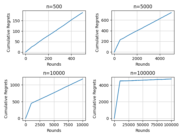
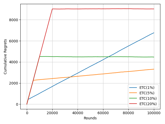
Figure 2 shows the performance of the ETC algorithm in different horizons with a 10% degree of exploration. There is an inflection point of each curve near the 10000th round which is the transition point from exploration to exploitation. With the increase of the horizon, the cumulative regret increases slowly because of the sufficiency of exploration. Figure 3 reflects the importance of the balance of exploration and exploitation. A proper degree of exploration can make the performance better.
4.2.2. SoftMax and Annealing SoftMax. The SoftMax algorithm is sensitive to the initial value of the average reward of each arm. Figure 4 shows the performance of the SoftMax become more and more better with the increase of the estimates. The performance is relatively better when the estimates are equal to 4 and the algorithm is initialized based on prior knowledge.
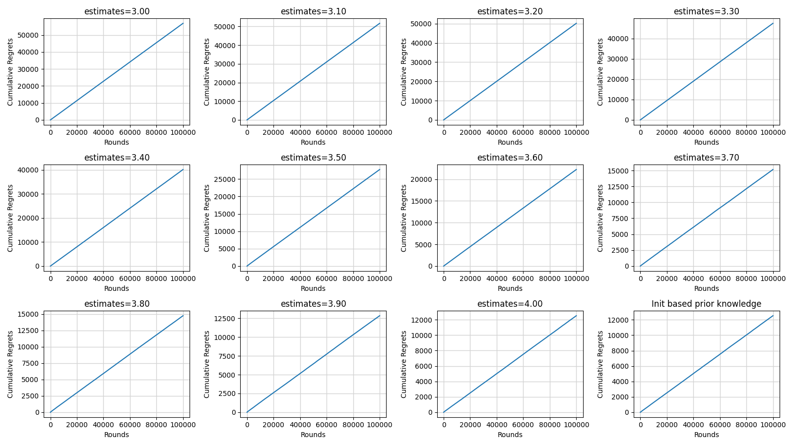
Figure 4. The cumulative regrets of the SoftMax algorithm with different initial values of the average reward of each arm (Photo/Picture credit: Original).
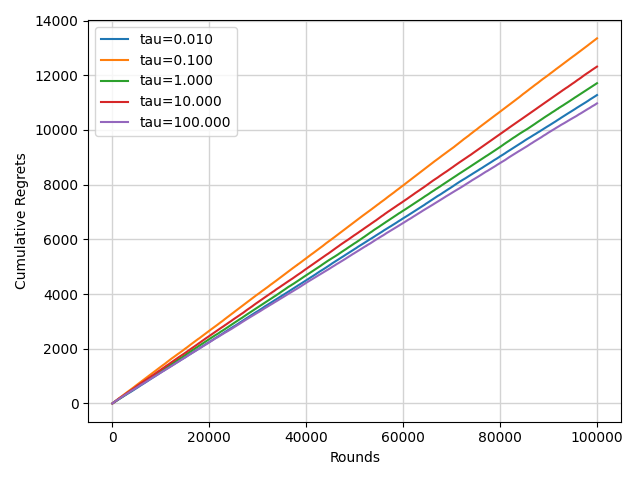
Figure 5. The cumulative regrets of SoftMax algorithm with different \( τ \) (Photo/Picture credit: Original).
Unlike the previous analysis, in this situation, the change in \( τ \) does not have an obvious impact on the performance of the SoftMax algorithm from Figure 5.
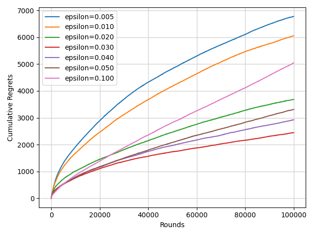
4.2.3. Epsilon Greedy and Annealing Epsilon Greedy. The choice of \( ϵ \) has a strong impact on the performance of the Epsilon Greedy algorithm from the observation of Figure 6. The algorithm's performance will suffer if \( ϵ \) is excessively high or little, as it won't be thoroughly explored or well exploited.
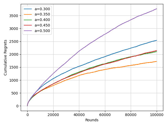
The annealing function \( f(t) \) the experiment chosen is the formula (3). The annealing Epsilon Greedy algorithm outperforms the normal one, as shown in Figure 7, with the best performance occurring when \( a \) equals to 0.35.
|
| |
Figure 6. The comparison of the performance of the Epsilon Greedy algorithm with different \( ϵ \) (Photo/ Picture credit: Original). | Figure 7. The comparison of the performance of Annealing Epsilon Greedy algorithm with different coefficient \( a \) (Photo/Picture credit: Original). |
4.2.4. Upper Confidence Bound and Variants. The formula of the UCB index in this experiment is.
\( UC{B_{i}}(t-1)={\hat{μ}_{i}}(t-1)+\frac{B}{2}\sqrt[]{\frac{llogn}{{T_{i}}(t-1)}} \) (10)
Where the \( l \) represent the balance between exploration and exploitation. The larger is the \( l \) value the more will the algorithm explore, while with smaller \( l \) it will more aggressively exploit. Through the observation of Figure 8, with the increase of \( l \) , the cumulative regret increases obviously.
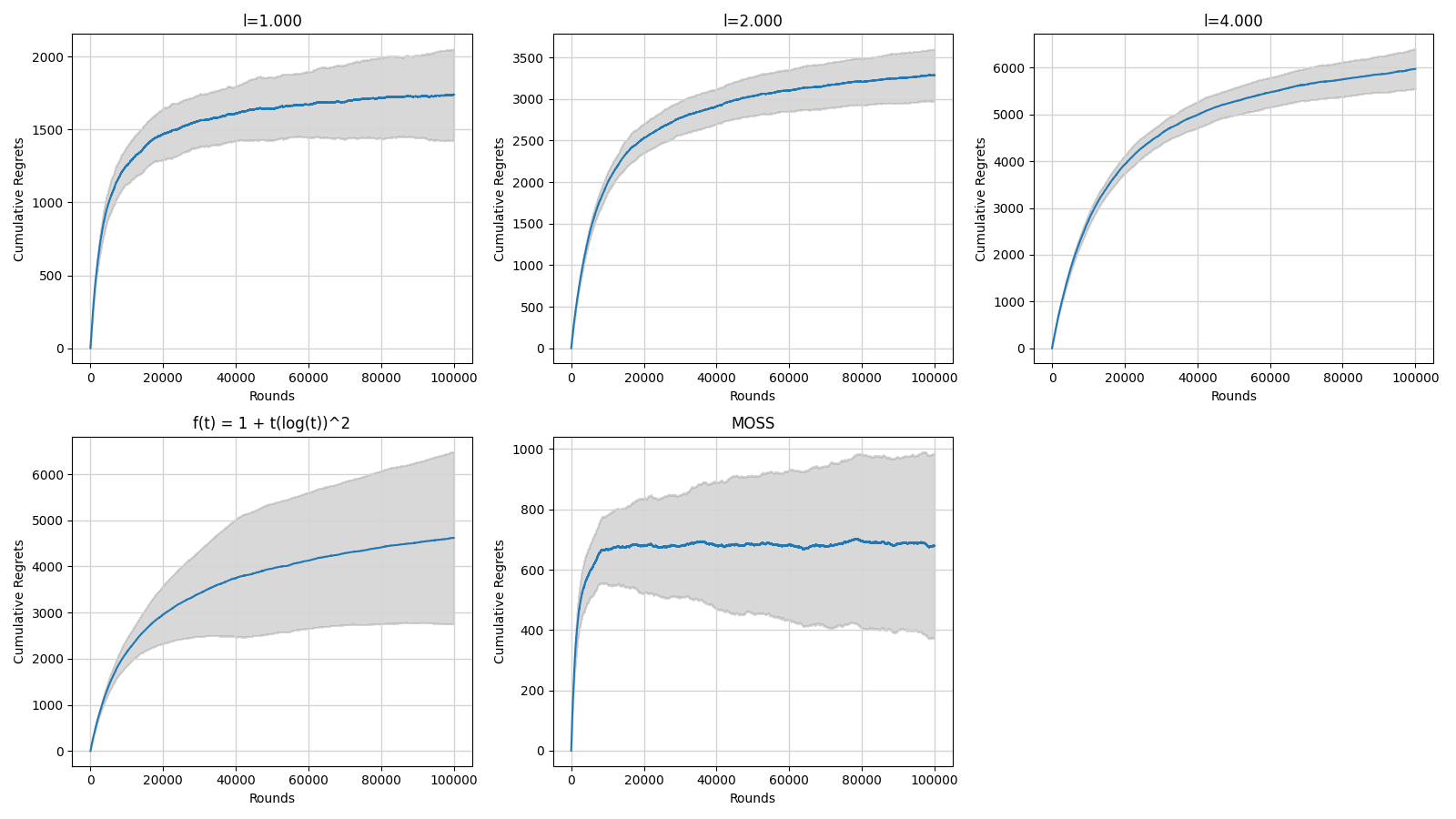
Figure 8. The comparison of the performance of UCB algorithm and its variants with error bars (Photo/Picture credit: Original).
Compared with the standard UCB algorithm, the asymptotically optimal UCB algorithm (first of the second line) and MOSS algorithm (second of the second line) have larger error bars. Compared to the UCB algorithm and the asymptotically optimal UCB algorithm, the MOSS algorithm performs better.
4.2.5. Thompson Sampling and Comparison. An understandable comparison of several multi-armed bandit algorithms may be seen in Figure 9. The ETC algorithm and the SoftMax algorithm do not have relatively good performance so they are not involved in the figure. In the figure 10, algorithms all have a \( O(log{n}) \) cumulative regrets. The Thompson Sampling has the best performance.
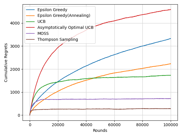
Figure 9. The comparison of the performance of different multi-armed bandit algorithms (Photo/Picture credit: Original).
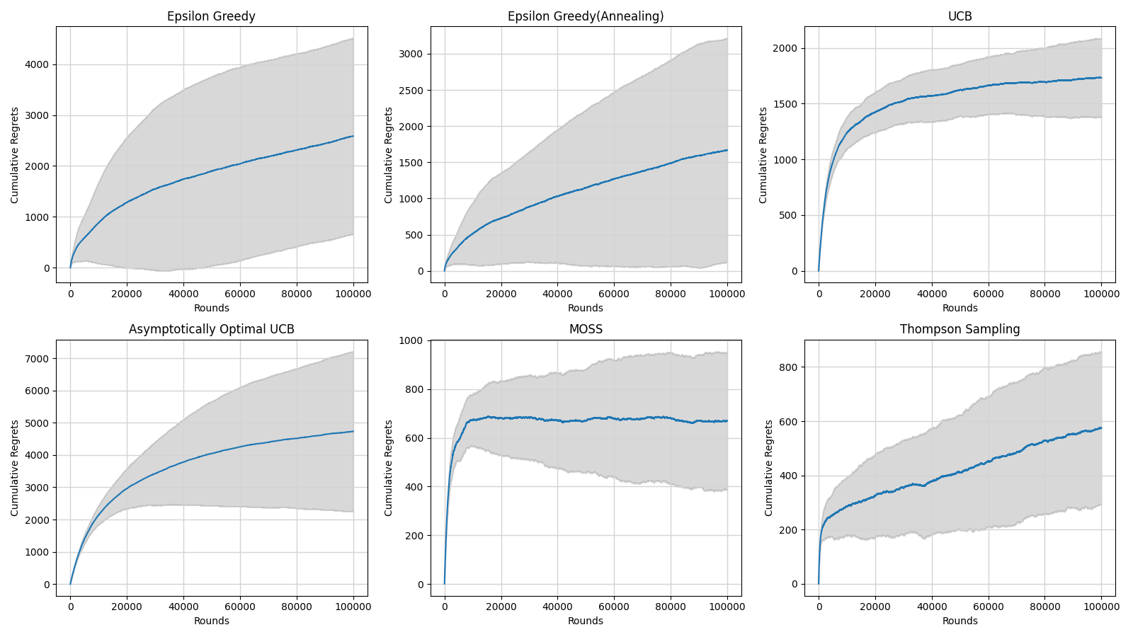
Figure 10. The comparison of the performance of different multi-armed bandit algorithms with error bars (Photo/Picture credit: Original).
Through the comparison of the width of the error bars of different algorithms, the Epsilon Greedy algorithm explores and exploits more randomly than other algorithms. The standard UCB algorithm is relatively stable. The MOSS algorithm and the Thompson Sampling algorithm have good performance among these algorithms.
4.3. Limitations of Classic Bandit Algorithms
Although classic bandit algorithms show strong performance in many scenarios, they still encounter several challenges and limitations when confronted with real-world complex environments:
Ignoring Contextual Information: Classical bandit algorithms do not take into account contextual information that may be present at each action point. This means that they do not take advantage of additional information associated with each action point. Consequently, they may underperform in situations where context plays a crucial role.
Inapplicability to Dynamic Environments: Classic bandit algorithms often suppose that the environment is stationary, which means the distribution of the reward of each arm does not change. However, in the real world, the environment is dynamic. The distribution is impacted by time, actions, and contextual information.
Missing action combinations: In some scenarios, the bandit algorithm needs to select a portfolio of actions to maximize the reward every round. The classic algorithm usually chooses one action per round. This limitation may restrict their ability to exploit potential synergies between different actions, resulting in suboptimal outcomes.
4.4. New Models and Approaches
To tackle the above problems with the classic bandit algorithm and fit the complex requirements in the real world, many researchers propose a lot of new models and approaches. These ideas aim to enhance the decision-making accuracy, adaptability, and efficiency in various applications based on the classic bandit algorithms. Here are some significant examples.
4.4.1. Contextual Bandits. In the real world, the contextual information cannot be ignored. Focusing on the experiments in this paper, the dataset has lots of contextual information such as users’ gender, age, and occupation. In a recommendation system, the assignment has been redesigned to suggest movies to users based on their past ratings. Such information affects the decision making of the agent to some extent. The Contextual Bandits focuses on such tasks. The agent considers the contextual information to adjust the policy when it makes a decision.
4.4.2. Combinatorial Bandits. Combinatorial bandits are an extension of the classic multi-armed bandit problem. The agent can select more than one action at once in place of just one at a time. In combinatorial bandits, actions are composed of combinations of individual choices. In each round, the player selects a combination of actions and observes the rewards associated with those choices, aiming to maximize cumulative reward.
4.5. Applications
4.5.1. Recommendation System In recent years, the Contextual Bandits model has been widely utilized in recommendation systems. In 2010, Li et al proposed the LinUCB algorithm to solve the news homepage recommendation problem. The LinUCB algorithm is initially proposed for linear return models. It achieves an efficient upper bound confidence algorithm by efficiently computing confidence intervals for the parameters. The LinUCB algorithm specifically looks at the scenario of a linear model first, such as one in which the expected reward and the characteristics have a linear connection. In this case, by applying ridge regression to the training data, the values of the parameters can be estimated and the corresponding upper bound confidence can be calculated. And Xu et al primarily utilized a contextual bandit algorithm to capture users' interest preferences over time.
4.5.2. Clinical Trail. This research [6] focuses on designing an Adaptive Clinical Trial (ACT) for animal experiments investigating cancer therapy effectiveness. The goal is to allocate treatments based on tumor volume data to improve outcomes while minimizing exposure to ineffective treatments. The study uses a contextual bandit approach, where treatments are selected based on prior data collected after completing groups of animals. By implementing the GP BESA strategy, the ACT showed improved longevity in mice compared to basic treatment strategies, demonstrating the effectiveness of adaptive treatment allocation in optimizing tumor growth outcomes. In order to solve the challenge of determining and giving a patient a suitable starting dose, Bastani et al modeled the issue as a multi-armed bandit problem with high-dimensional variables. They then suggested a creative and effective multi-armed bandit approach that was based on the LASSO estimator.
The research proposes a contextual bandit algorithm that dynamically optimizes treatment selection during the trial by considering patient characteristics. The algorithm is evaluated using real clinical trial data from the International Stroke Trial and is compared to random assignment and a context-free multi-arm bandit approach. The results indicate that the contextual-bandit approach outperforms the other methods, providing substantial gains in assigning the most suitable treatments to participants.
4.5.3. Financial Investment. To create a pool of candidate portfolios, the study suggests a two-stage investment technique that combines the LinUCB algorithm to generate a portfolio update rule based on a particular utility function with a supervised adaptive decision tree approach. The goal of the research is to strike a balance between exploration and exploitation when choosing a portfolio, taking into account investors' erratic tastes for various assets.
The research focuses on online portfolio selection problems in both full-feedback and bandit-feedback settings. The study introduces algorithms with sublinear regret upper bounds and analyzes regret lower bounds for these settings. The algorithms combine the multiplicative weight update method (MWU) or multi-armed bandit algorithms (MAB) with online convex optimization (OCO) techniques.
5. Conclusion
This work compares the effectiveness of many traditional stochastic multi-armed bandit algorithms and discusses several new multi-armed bandit issue models and their usage.
In the experiment part, different classic stochastic multi-armed bandit algorithms are implemented. The ETC algorithm is a simple algorithm that is easy to understand and implement. However, it needs to know the horizon and it is hard to determine the degree of exploration. The SoftMax algorithm refers to a physical idea but it is sensitive to the initialization. The Epsilon Greedy algorithm has a relatively good balance of exploration and exploitation by adjusting the value of \( ϵ \) and the idea of annealing further improves its performance. The UCB algorithm and its variants concentrate on the choice of the formula to calculate the UCB index. Different designs for calculating the UCB index impact the performance and the MOSS algorithm has better performance. Thompson Sampling is based on the Bayesian inference balancing exploration and exploitation and shows the best performance among all algorithms.
In the discussion part, contextual bandits and combinatorial bandit algorithms are introduced. They can adapt to the real world and more complex environments better. Some contextual are considered and combinations of arms are given when the algorithm takes an action. There are lots of applications of multi-armed bandit algorithms. In recommendation systems, a variant of the UCB algorithm with the idea of contextual bandits called the LinUCB algorithm is introduced to solve the problem of news homepage recommendation. The multi-armed bandit algorithms are also used in the medical field to conduct clinical trials. They are also used by financial experts to select good financial portfolios.
This study provides valuable insights into multi-armed bandit algorithms, aiding both academia and industry. By comparing classic approaches and introducing new models, it equips practitioners with actionable knowledge for decision-making in diverse domains. Future research may focus on refining algorithms for scalability and adaptability. Interdisciplinary collaborations can drive innovation, enhancing the applicability of these algorithms in dynamic environments. Overall, this work lays the foundation for continued advancements in sequential decision-making methodologies, with wide-ranging implications for various sectors.
References
[1]. Li, L., Chu, W., Langford, J., & Schapire, R. E. (2010, April). A contextual-bandit approach to personalized news article recommendation. In Proceedings of the 19th international conference on World wide web (pp. 661-670).1.
[2]. Said, A., Berkovsky, S., De Luca, E. W., & Hermanns, J. (2011, October). Challenge on context-aware movie recommendation: CAMRa2011. In Proceedings of the fifth ACM conference on Recommender systems (pp. 385-386).
[3]. Xu, X., Dong, F., Li, Y., He, S., & Li, X. (2020, April). Contextual-bandit based personalized recommendation with time-varying user interests. In Proceedings of the AAAI Conference on Artificial Intelligence (Vol. 34, No. 04, pp. 6518-6525).
[4]. Yan, C., Xian, J., Wan, Y., & Wang, P. (2021). Modeling implicit feedback based on bandit learning for recommendation. Neurocomputing, 447, 244-256.
[5]. Gan, M., & Kwon, O. C. (2022). A knowledge-enhanced contextual bandit approach for personalized recommendation in dynamic domains. Knowledge-Based Systems, 251, 109158.
[6]. Durand, A., Achilleos, C., Iacovides, D., Strati, K., Mitsis, G. D., & Pineau, J. (2018, November). Contextual bandits for adapting treatment in a mouse model of de novo carcinogenesis. In Machine learning for healthcare conference (pp. 67-82). PMLR.
[7]. Bastani, H., & Bayati, M. (2020). Online decision making with high-dimensional covariates. Operations Research, 68(1), 276-294.
[8]. Varatharajah, Y., & Berry, B. (2022). A contextual-bandit-based approach for informed decision-making in clinical trials. Life, 12(8), 1277.
[9]. Shen, W., Wang, J., Jiang, Y. G., & Zha, H. (2015, June). Portfolio choices with orthogonal bandit learning. In Twenty-fourth international joint conference on artificial intelligence.
[10]. Moeini, M. (2019). Orthogonal bandit learning for portfolio selection under cardinality constraint. In Computational Science and Its Applications–ICCSA 2019: 19th International Conference, Saint Petersburg, Russia, July 1–4, 2019, Proceedings, Part III 19 (pp. 232-248). Springer International Publishing.
[11]. Charpentier, A., Elie, R., & Remlinger, C. (2021). Reinforcement learning in economics and finance. Computational Economics, 1-38.
[12]. Ni, H., Xu, H., Ma, D., & Fan, J. (2023). Contextual combinatorial bandit on portfolio management. Expert Systems with Applications, 221, 119677.
[13]. Angelelli, E., Mansini, R., & Speranza, M. G. (2012). Kernel search: A new heuristic framework for portfolio selection. Computational Optimization and Applications, 51, 345-361.
[14]. Ito, S., Hatano, D., Sumita, H., Yabe, A., Fukunaga, T., Kakimura, N., & Kawarabayashi, K. I. (2018). Regret bounds for online portfolio selection with a cardinality constraint. Advances in Neural Information Processing Systems, 31.
[15]. Huo, X., & Fu, F. (2017). Risk-aware multi-armed bandit problem with application to portfolio selection. Royal Society open science, 4(11), 171377.
[16]. Lu, T., Pál, D., & Pál, M. (2010, March). Contextual multi-armed bandits. In Proceedings of the Thirteenth international conference on Artificial Intelligence and Statistics (pp. 485-492). JMLR Workshop and Conference Proceedings.
[17]. Li, C., & Wang, H. (2022, May). Asynchronous upper confidence bound algorithms for federated linear bandits. In International Conference on Artificial Intelligence and Statistics (pp. 6529-6553). PMLR.
[18]. Pacchiano, A., Ghavamzadeh, M., Bartlett, P., & Jiang, H. (2021, March). Stochastic bandits with linear constraints. In International conference on artificial intelligence and statistics (pp. 2827-2835). PMLR.
[19]. Ding, Q., Hsieh, C. J., & Sharpnack, J. (2021, March). An efficient algorithm for generalized linear bandit: Online stochastic gradient descent and thompson sampling. In International Conference on Artificial Intelligence and Statistics (pp. 1585-1593). PMLR.
[20]. Cella, L., Lazaric, A., & Pontil, M. (2020, November). Meta-learning with stochastic linear bandits. In International Conference on Machine Learning (pp. 1360-1370). PMLR.
[21]. Zhu, X., Huang, Y., Wang, X., & Wang, R. (2023). Emotion recognition based on brain-like multimodal hierarchical perception. (pp. 1-19). Multimedia Tools and Applications.
[22]. Wang, H., Yang, Y., Wang, E., Liu, W., Xu, Y., & Wu, J. (2020, June). Combinatorial multi-armed bandit based user recruitment in mobile crowdsensing. In 2020 17th Annual IEEE International Conference on Sensing, Communication, and Networking (SECON) (pp. 1-9). IEEE.
[23]. Gao, G., Huang, H., Xiao, M., Wu, J., Sun, Y. E., & Zhang, S. (2021, May). Auction-based combinatorial multi-armed bandit mechanisms with strategic arms. In IEEE INFOCOM 2021-IEEE Conference on Computer Communications (pp. 1-10). IEEE.
Cite this article
Fei,B. (2024). Comparative analysis and applications of classic multi-armed bandit algorithms and their variants. Applied and Computational Engineering,68,17-30.
Data availability
The datasets used and/or analyzed during the current study will be available from the authors upon reasonable request.
Disclaimer/Publisher's Note
The statements, opinions and data contained in all publications are solely those of the individual author(s) and contributor(s) and not of EWA Publishing and/or the editor(s). EWA Publishing and/or the editor(s) disclaim responsibility for any injury to people or property resulting from any ideas, methods, instructions or products referred to in the content.
About volume
Volume title: Proceedings of the 6th International Conference on Computing and Data Science
© 2024 by the author(s). Licensee EWA Publishing, Oxford, UK. This article is an open access article distributed under the terms and
conditions of the Creative Commons Attribution (CC BY) license. Authors who
publish this series agree to the following terms:
1. Authors retain copyright and grant the series right of first publication with the work simultaneously licensed under a Creative Commons
Attribution License that allows others to share the work with an acknowledgment of the work's authorship and initial publication in this
series.
2. Authors are able to enter into separate, additional contractual arrangements for the non-exclusive distribution of the series's published
version of the work (e.g., post it to an institutional repository or publish it in a book), with an acknowledgment of its initial
publication in this series.
3. Authors are permitted and encouraged to post their work online (e.g., in institutional repositories or on their website) prior to and
during the submission process, as it can lead to productive exchanges, as well as earlier and greater citation of published work (See
Open access policy for details).
References
[1]. Li, L., Chu, W., Langford, J., & Schapire, R. E. (2010, April). A contextual-bandit approach to personalized news article recommendation. In Proceedings of the 19th international conference on World wide web (pp. 661-670).1.
[2]. Said, A., Berkovsky, S., De Luca, E. W., & Hermanns, J. (2011, October). Challenge on context-aware movie recommendation: CAMRa2011. In Proceedings of the fifth ACM conference on Recommender systems (pp. 385-386).
[3]. Xu, X., Dong, F., Li, Y., He, S., & Li, X. (2020, April). Contextual-bandit based personalized recommendation with time-varying user interests. In Proceedings of the AAAI Conference on Artificial Intelligence (Vol. 34, No. 04, pp. 6518-6525).
[4]. Yan, C., Xian, J., Wan, Y., & Wang, P. (2021). Modeling implicit feedback based on bandit learning for recommendation. Neurocomputing, 447, 244-256.
[5]. Gan, M., & Kwon, O. C. (2022). A knowledge-enhanced contextual bandit approach for personalized recommendation in dynamic domains. Knowledge-Based Systems, 251, 109158.
[6]. Durand, A., Achilleos, C., Iacovides, D., Strati, K., Mitsis, G. D., & Pineau, J. (2018, November). Contextual bandits for adapting treatment in a mouse model of de novo carcinogenesis. In Machine learning for healthcare conference (pp. 67-82). PMLR.
[7]. Bastani, H., & Bayati, M. (2020). Online decision making with high-dimensional covariates. Operations Research, 68(1), 276-294.
[8]. Varatharajah, Y., & Berry, B. (2022). A contextual-bandit-based approach for informed decision-making in clinical trials. Life, 12(8), 1277.
[9]. Shen, W., Wang, J., Jiang, Y. G., & Zha, H. (2015, June). Portfolio choices with orthogonal bandit learning. In Twenty-fourth international joint conference on artificial intelligence.
[10]. Moeini, M. (2019). Orthogonal bandit learning for portfolio selection under cardinality constraint. In Computational Science and Its Applications–ICCSA 2019: 19th International Conference, Saint Petersburg, Russia, July 1–4, 2019, Proceedings, Part III 19 (pp. 232-248). Springer International Publishing.
[11]. Charpentier, A., Elie, R., & Remlinger, C. (2021). Reinforcement learning in economics and finance. Computational Economics, 1-38.
[12]. Ni, H., Xu, H., Ma, D., & Fan, J. (2023). Contextual combinatorial bandit on portfolio management. Expert Systems with Applications, 221, 119677.
[13]. Angelelli, E., Mansini, R., & Speranza, M. G. (2012). Kernel search: A new heuristic framework for portfolio selection. Computational Optimization and Applications, 51, 345-361.
[14]. Ito, S., Hatano, D., Sumita, H., Yabe, A., Fukunaga, T., Kakimura, N., & Kawarabayashi, K. I. (2018). Regret bounds for online portfolio selection with a cardinality constraint. Advances in Neural Information Processing Systems, 31.
[15]. Huo, X., & Fu, F. (2017). Risk-aware multi-armed bandit problem with application to portfolio selection. Royal Society open science, 4(11), 171377.
[16]. Lu, T., Pál, D., & Pál, M. (2010, March). Contextual multi-armed bandits. In Proceedings of the Thirteenth international conference on Artificial Intelligence and Statistics (pp. 485-492). JMLR Workshop and Conference Proceedings.
[17]. Li, C., & Wang, H. (2022, May). Asynchronous upper confidence bound algorithms for federated linear bandits. In International Conference on Artificial Intelligence and Statistics (pp. 6529-6553). PMLR.
[18]. Pacchiano, A., Ghavamzadeh, M., Bartlett, P., & Jiang, H. (2021, March). Stochastic bandits with linear constraints. In International conference on artificial intelligence and statistics (pp. 2827-2835). PMLR.
[19]. Ding, Q., Hsieh, C. J., & Sharpnack, J. (2021, March). An efficient algorithm for generalized linear bandit: Online stochastic gradient descent and thompson sampling. In International Conference on Artificial Intelligence and Statistics (pp. 1585-1593). PMLR.
[20]. Cella, L., Lazaric, A., & Pontil, M. (2020, November). Meta-learning with stochastic linear bandits. In International Conference on Machine Learning (pp. 1360-1370). PMLR.
[21]. Zhu, X., Huang, Y., Wang, X., & Wang, R. (2023). Emotion recognition based on brain-like multimodal hierarchical perception. (pp. 1-19). Multimedia Tools and Applications.
[22]. Wang, H., Yang, Y., Wang, E., Liu, W., Xu, Y., & Wu, J. (2020, June). Combinatorial multi-armed bandit based user recruitment in mobile crowdsensing. In 2020 17th Annual IEEE International Conference on Sensing, Communication, and Networking (SECON) (pp. 1-9). IEEE.
[23]. Gao, G., Huang, H., Xiao, M., Wu, J., Sun, Y. E., & Zhang, S. (2021, May). Auction-based combinatorial multi-armed bandit mechanisms with strategic arms. In IEEE INFOCOM 2021-IEEE Conference on Computer Communications (pp. 1-10). IEEE.