1 Introduction

The rapid progress in the field of artificial intelligence, especially deep learning technology [1], has led to an emerging research field: the use of deep learning to solve traditional scientific computing problems [2]. In this field, researchers use artificial intelligence technology to learn and simulate scientific laws in nature, which are traditionally described by complex mathematical equations. Through deep learning, researchers have found innovative solutions and opportunities in scientific computing problems that cannot be efficiently solved by traditional methods. This not only promotes the progress of scientific computing, but also expands new boundaries for the application of deep learning technology.

This article introduces in detail the current basic methods and traditional models for solving scientific computing problems through Physics-Informed Neural Networks (PINNs) embedded [3] with physical information [4], and discusses the challenges faced by new numerical methods using PINNs to solve partial differential equations [5]. In addition, this paper introduces in-depth solutions to common partial differential equations by introducing Ordinary Differential Equation Networks (ODE-Nets) as the network layer and combining some advanced training techniques used in the solution process. This method not only improves the solution accuracy, but also enhances the generalization ability of the model, providing an efficient new solution strategy for complex scientific computing problems.

2 Related works

2.1 Advantages and limitations of PINN in numerical calculation problems

Physics-Informed Neural Networks (PINN) is an innovative model that integrates traditional physics theory and modern machine learning technology. It uses a deep learning framework to solve physical problems, especially partial differential equations. The core advantage of the PINN model is that it naturally avoids the grid processing necessary in traditional numerical calculation methods. This feature enables it to demonstrate significant flexibility and computational efficiency when processing complex-shaped or multi-dimensional physical scenes.

Specifically, PINN shows higher adaptability and scalability than traditional methods for handling application scenarios that do not require precise meshing. This is particularly important when solving partial differential equations in high-dimensional spaces, where meshing is computationally expensive and intractable.

In addition, PINN has also shown excellent application potential in reverse engineering problems [6], especially in parameter estimation and model correction. By appropriately adjusting the network structure and weights, PINN can directly estimate unknown parameters. This process does not rely on a large amount of experimental data, providing an effective solution for scenarios where data is scarce or experiments are expensive.

However, despite its outstanding performance in many aspects, PINN still faces a series of challenges. The most important ones are training costs and convergence issues [7]. Physics-informed neural networks often need to be retrained when encountering new physical conditions or problem changes, a process that is time-consuming and expensive. Furthermore, an efficient training process requires careful balancing of the various parts of the equation, often by adjusting trade-off parameters λ to achieve. If λ is not set appropriately, the model may overemphasize certain equation parts and ignore other key physical behaviors, thus affecting the model’s learning effect and prediction accuracy.

Consider a simple example such as the wave equation:

\( \frac{∂^{2}u(x,t)}{∂t^{2}}-c^{2}\frac{∂^{2}u(x,t)}{∂t^{2}}=0 (1) \)

\( u(x,t=0)=f(x), \frac{∂u}{∂t}(x,t=0)=g(x) (2) \)

\( u(x=0,t)=u(x=l)=0 (3) \)

At this time, the loss function of the PINN is:

\( L_{PDE}=\frac{1}{M}\sum_{i=0}^{M}(\hat{u}_{tt}(x_{i},t_{i})-c^{2}\hat{u}_{tt}(x_{i},t_{i}))^{2} (5) \)

\( L_{initial}=\frac{1}{P}\sum_{j=1}^{P}\lbrace (\hat{u}(0,x_{i})-f(x_{j}))^{2}+(\frac{∂\hat{u}}{∂t}(0,x_{i})-g(x_{j}))^{2}\rbrace (6) \)

\( L_{iniboundary}=\frac{1}{Q}\sum_{k=0}^{Q}\lbrace (\hat{u}(x=0,t_{k}))^{2}+(\hat{u}(x=l,t_{k}))^{2}\rbrace (7) \)

\( Loss=L_{PDE}+L_{initial}+L_{iniboundary} \)

As can be seen from above formulas, when using a neural network to approximate a multivariate function through embedded physical information, the neural network uˆ appears multiple times. It can be regarded as using uˆtt(xi, ti). The time second-order derivative network approximates the displacement second-order derivative network c2uˆxx(xi, ti), which leads to correlation between the data and thus destabilizes the training network, which explains the poor convergence of the PINN.

2.2 Neural Ordinary Differential Equations

Neural Ordinary Differential Equations (Neural ODEs for short) is a deep learning model that simulates the behavior of continuous dynamic systems by combining ordinary differential equations (ODEs) with neural networks. This model was first proposed by Chen et al. in 2018 and is an innovation in the field of deep learning.

It gives a novel perspective on traditional residual neural networks, Consider a residual neural network. For the layer, we can use the following expression to describe:

\( h(t+1)=h(t)+f(h(t);θ_{t}) (8) \)

Through some simple transformations you can get

\( h(t+1)-h(t)=f(h(t);θ_{t}) \) \( (9) \)

\( \frac{h(t+1)-h(t)}{1}=f(h(t);θ_{t}) (10) \)

By reducing the layer interval in ResNet to the limit, it can be regarded as a continuous neural network, which is the core idea of Neural ODE. This approach allows us to contrast the discrete structure of ResNet with its continuous form. In the continuous neural network model, the change of the system state is controlled by a time-invariant nonlinear function, which is very similar to the structure of an ordinary differential equation (ODE).

\( \frac{h(t+1)-h(t)}{∆t}=f(h(t);θ_{t}) (11) \)

\( \frac{∆h}{∆t}=f(h(t);θ_{t}) (12) \)

\( \frac{dh}{dt}=f(h(t);θ_{t}) (13) \)

This allows us to use the micro -division equation to find out the output between the network layer.

\( \int_{h(t)}^{h(t+1)}h(t)=\int_{t}^{t+1}f(h(t);θ_{t}) (14) \)

This means that the form of the loss function will become

\( L\lbrace z(t+1)\rbrace =L\lbrace z(t)+\int_{t}^{t+1}f(z(t);θ_{t};t)dt\rbrace =L\lbrace ODESolve(z(t+1);f;t;t+1;θ_{t})\rbrace \) \( (15) \)

Under the network layer designed in this way, the adjoint method can be used to achieve backward of the network.

In application scenarios where continuous dynamic systems need to be simulated, divine constant differential equations show more powerful performance than traditional discrete-time neural network models.

3 Methodology

The current study has explored in detail the operation mechanism of Physical Information Neural Networks (PINNs), and based on this, this paper proposes an innovative network architecture, ODENet-PINN, which incorporates the features of Ordinary Differential Equation Networks (ODENet), especially the advantages in modeling continuous time series dynamical systems, to enhance the efficiency and accuracy of solving partial differential equations. The architecture incorporates the features of the Ordinary Differential Equation Network (ODENet), especially in modeling continuous time series dynamical systems, to enhance the efficiency and accuracy of solving partial differential equations.

The core strength of ODENet, a neural network architecture dedicated to solving dynamic system simulation problems, lies in its ability to accurately simulate the evolution of the system state through adaptive time steps. This feature makes ODENet well suited to deal with complex problems that require continuous-time modeling, such as fluid dynamics and heat transfer problems.Combined with physically-informed neural networks, ODENet-PINN is not only able to leverage ODENet’s strengths in dynamic system simulation, but also directly integrates the laws of physics as part of the training process through the framework of PINN, thus ensuring the physical interpretability of the solution process and the accuracy of the results.

Through comparative experiments, this study found that ODENetPINN performs well in solving partial differential equations. Compared with traditional fully connected neural networks (FCNN) or residual neural networks (ResNet), ODENet-PINN not only shows significant improvement in generalization ability, but also demonstrates advantages in the stability of network training and convergence speed. In addition, we introduce a new training technique to enhance the stability of the training process by fixing the target network parameters, which improves the convergence of the network and the robustness of the model.

4 Experiments

4.1 Experimental scene

The experiments consider using the three most classic equations in mathematical physics equations: wave equation, heat conduction equation, and Laplace equation as our solution objects.

The wave equation is a partial differential equation used to describe the phenomenon of wave propagation or vibration. It was originally used to explain the propagation behavior of sound waves, water waves, light waves and electromagnetic waves, and constitutes one of the basic theories of physics. The typical form of the wave equation consists of the second-order derivatives in time and space, describing the relationship between the wave function changing with time and space. In the field of modern science and engineering, the wave equation is widely used in acoustics, seismology, optics, electromagnetics, structural analysis, water wave simulation and quantum mechanics. It is an important tool for studying and simulating wave propagation, vibration phenomena and related interactions.

\( \frac{∂^{2}u}{∂t^{2}}=c^{2}∇^{2}u (16) \)

The heat conduction equation is a partial differential equation that describes the propagation of heat in a medium. It was proposed by the French mathematician Fourier in the 19th century and provides the basis for the theory of thermodynamics. This equation describes the relationship between thermal diffusion coefficient and temperature gradient, has smooth mathematical properties, and can explain the trend of the temperature field changing with time. In fields such as materials engineering, environmental science, biomedicine, energy engineering, electronics and semiconductors, and construction engineering, the heat conduction equation is used to simulate and optimize heat transfer and guide processes such as industrial processing, energy-saving design, and medical treatment.

\( \frac{∂u}{∂t}=α∇^{2}u (17) \)

Laplace’s equation is a partial differential equation that describes the characteristics of steady-state field distribution. It is used to describe the potential field distribution in the steady state. It is widely used in fields such as electromagnetism, fluid mechanics, and thermodynamics, such as simulating electric and magnetic fields, analyzing the pressure distribution of irrotational incompressible fluids, and describing the steady-state temperature field. In fields, such as structural engineering and image processing, Laplace’s equation is also used to study structural stress and image repair, and is an important tool in physics, engineering and computational science.

For the above three equations are used to solve the following initial conditions and boundary conditions:

\( \frac{∂^{2}u}{∂t^{2}}=c^{2}∇^{2}u (18) \)

\( u(0,x,y)=sin{(2πx)sin{(2πy) (19)}} \)

\( u(t,0,0)=u(t,1,0)=u(t,0,1)=u(t,1,1)=0 (20) \)

\( \frac{∂^{2}u}{∂t^{2}}=c^{2}∇^{2}u (21) \)

\( u(0,x,y)=sin{(πx)sin{(πy) (22)}} \)

\( u(0,x,y)=u(1,y,y)=u(x,0,t)=u(x,1,t)=0 (23) \)

\( ∇^{2}u=0 (24) \)

\( u(0,y)=sin{(πy) (25)} \)

\( u(1,y)=u(x,0)=u(x,1)=0 (26) \)

4.2 Environment of Experiments

In terms of model training, this study used high-performance computing resources to conduct a systematic comparative study on the baseline model fully connected neural network [8], residual neural network and improved model ODE-Net. All three models use the Adam optimizer, with the initial learning rate set to 0.001, and combined with a learning rate decay strategy to optimize the training process. Specifically, this study solved the three partial differential equations mentioned above by allowing the three models to have almost the same number of parameters and experimental data, and compared the solution results with the finite difference method implemented using numpy method to compare results. And for the three models, we only trained for 5000 epochs to judge the quality of the model.

4.3 Discussion and evaluation of Experiments

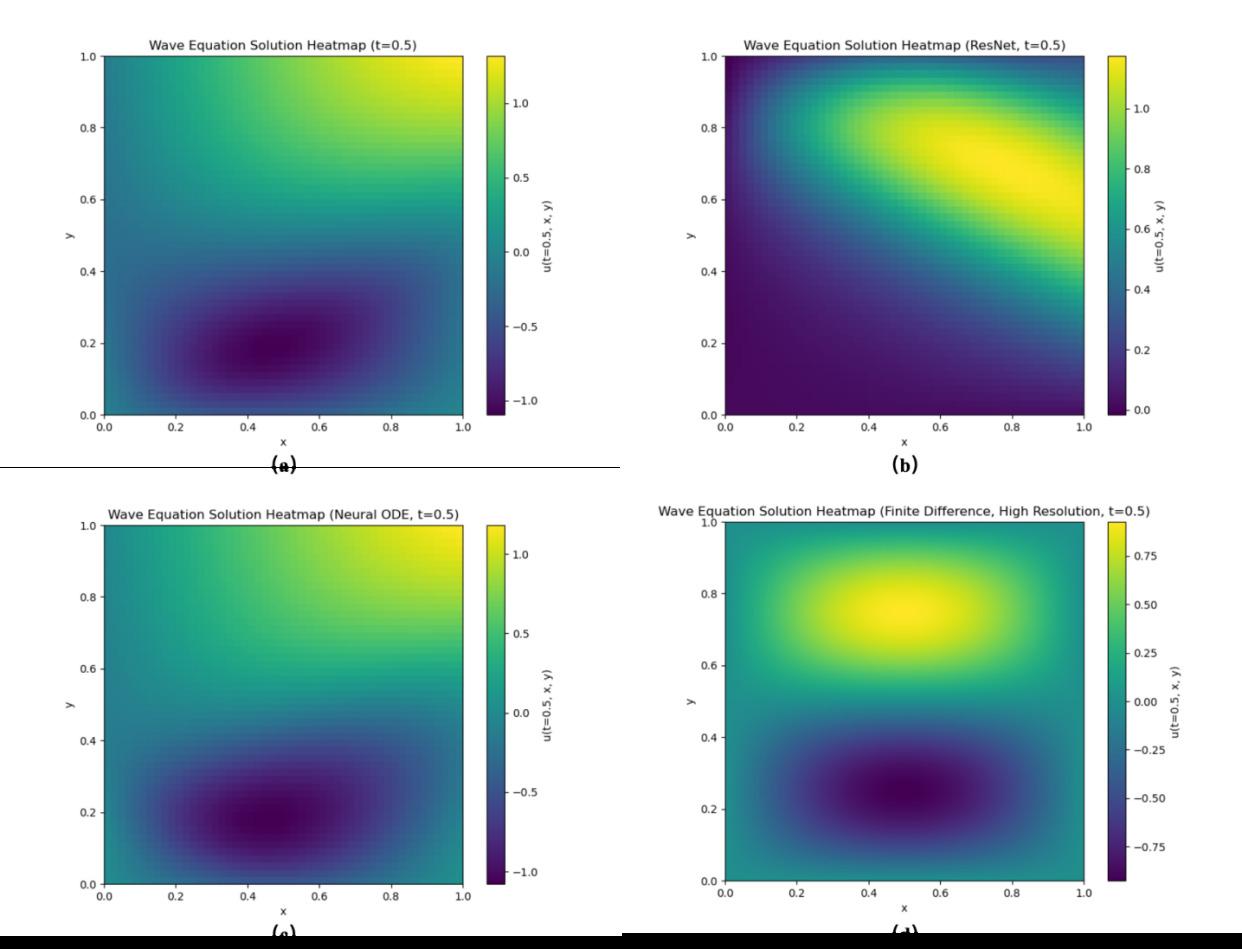
Figure 1. The prediction results of three models for the wave equation at t = 0.5 are shown: (a) the prediction results of the fully connected neural network, (b) the prediction results of the residual neural network, (c) the prediction results of the ODE-Net, and (d) the true results computed by finite difference method.

Experimental results show that the performance of fully connected neural networks, residual neural networks and ODE-Net on the wave equation is not ideal. This study speculate that this may be because 5000 epochs cannot fully train these networks, causing them to fail to generalize the solution well, making it difficult to accurately capture the dynamic characteristics of the wave equation. However, even with these limitations, the results still show that among the three networks, ODE-Net exhibits the best performance, especially when dealing with complex dynamic problems. This shows that the architecture of ODE-Net can better capture the characteristics and behavior of equations, making it more efficient and accurate in numerically solving such equations. In order to further improve the generalization ability of these networks, extending the training time or introducing more optimized training strategies can be considered in the future to improve their performance on the wave equation.

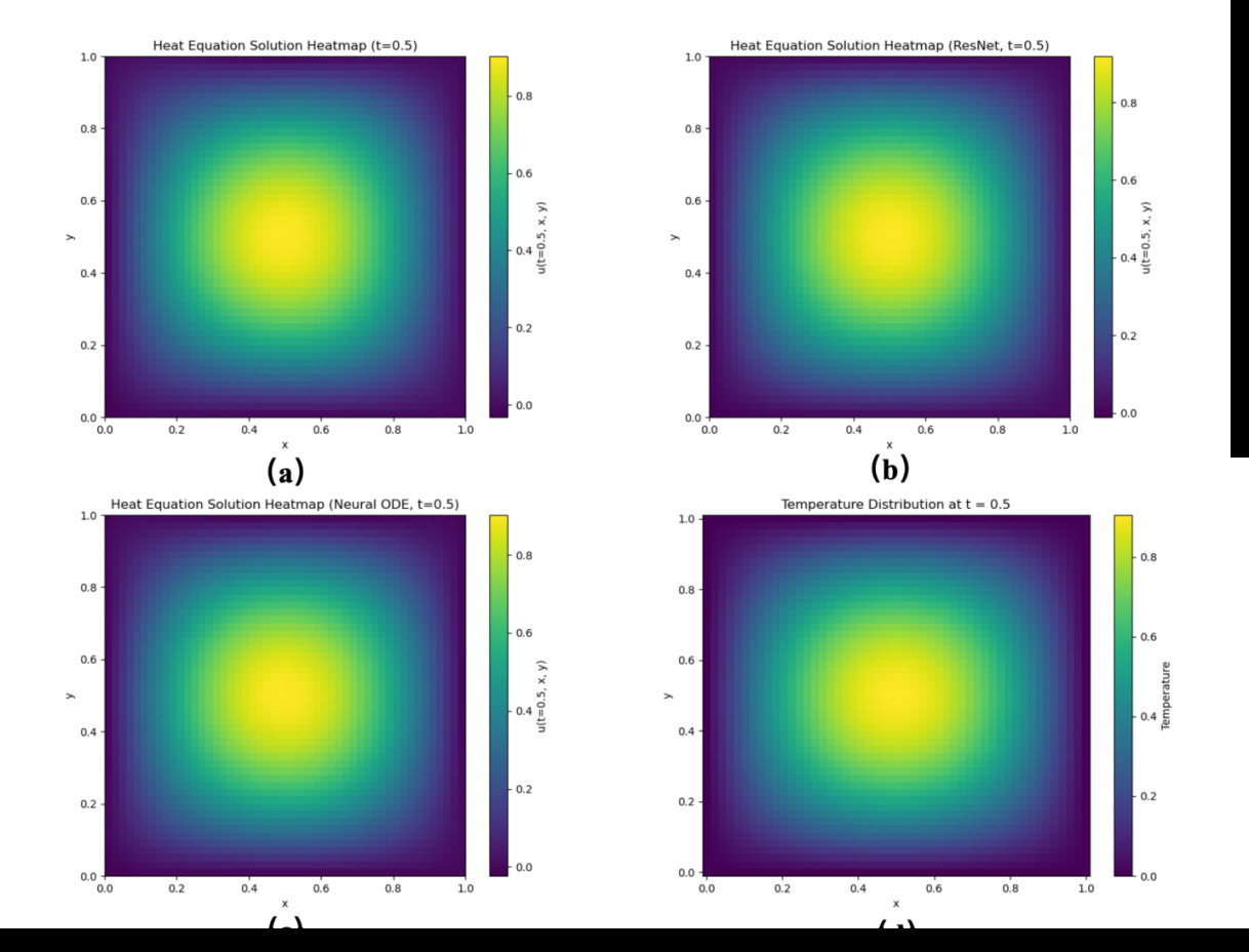
Figure 2. The prediction results of three models for the hight conduction equation at t = 0.5 are shown: (a) the prediction results of the fully connected neural network, (b) the prediction results of the residual neural network, (c) the prediction results of the ODE-Net, and (d) the true results computed by finite difference method.

In experiments on the heat conduction equation and the Laplace equation, all three networks showed good generalization capabilities, which may be related to the fact that the structure of the equation itself makes the network easier to converge. However, although they perform well in these two equations, there is still a certain gap compared with traditional numerical methods. It is worth noting that among these three types of networks, ODE-Net still exhibits the best generalization performance, indicating that it has significant advantages in capturing the characteristics of these equations and solving numerical problems.

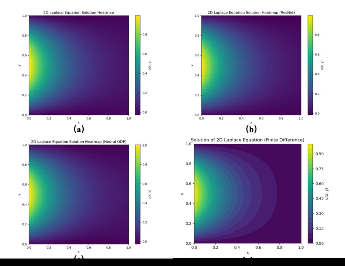
Figure 3. The prediction results of three models for the laplace equation at t =0.5 are shown: (a) the prediction results of the fully connected neural network, (b) the prediction results of the residual neural network, (c) the prediction results of the ODE-Net, and (d) the true results computed by finite difference method.

aken together, although the performance of fully connected neural networks and residual neural networks in solving different equations is acceptable, they are still slightly inefficient compared with ODE-Net. By further optimizing the training strategy and architecture design, the generalization ability of the ODENet network can be further developed, but appropriate training strategies need to be developed based on the characteristics of different equations to unleash their full potential.

5 Conclusion

The ablation experiments compared the performance of deep neural network models introducing residual networks [9] and ODE-Net with traditional fully connected neural networks in solving partial differential equations. At the same time, this study also compared the performance of these deep learning models with classic numerical methods. Experimental results show that deep learning models with complex network structures can not only significantly improve the solution accuracy when solving such mathematical problems, but also enhance the model’s adaptability and generalization to different problems. These findings effectively support the application of deep learning technology in the field of scientific computing and provide new research perspectives.

In particular, our research found that the neural network model added to ODE-Net [10] showed excellent fitting ability and generalization performance. Compared with traditional fully connected neural networks and residual neural networks, ODE-Net shows more powerful potential.

The results of this study show that by embedding the ODE-Net layer in the physical information neural network, the fitting ability and generalization performance of PINNs can be significantly enhanced. This discovery provides a new research direction for subsequent research on PINNs and points out potential ways to apply deep learning technology in the field of AI for Science to achieve better results. Our research not only promotes the integration of scientific computing and deep learning, but also opens up new possibilities for using deep learning to solve complex physical problems.

This study explored the use of neural networks, particularly ODE-Net embedded within Physics-Informed Neural Networks (PINNs), to solve partial differential equations. It conducted comparative experiments involving fully connected neural networks, residual neural networks, and ODE-Net across three classic mathematical physics equations: the wave equation, the heat conduction equation, and Laplace’s equation.

The experimental results demonstrated that, despite the generalization performance limitations on the wave equation due to the relatively short training epochs, ODE-Net still displayed superior filtering and generalization capabilities.This highlights ODE-Net’s architectural strength in modeling the characteristics and behaviors of equations, particularly in capturing complex dynamic phenomena. On the heat conduction and Laplace equations, all three network architectures showed good convergence, although ODE-Net once again exhibited the best overall generalization performance, indicating its notable advantage in simulating these equations.

Overall, the research provides a promising direction for further enhancing the efficacy of PINNs by embedding ODE-Net layers. This not only improves the fitting and generalization performance of these networks but also facilitates their ability to solve complex scientific computing problems. Future work could focus on optimizing training strategies and designing more specialized network architectures based on the unique characteristics of each equation, thereby enabling neural networks to reach their full potential in scientific computing.

References

[1]. Md. Zahangir Alom et al. (2019) “A State-of-the-Art Survey on Deep Learning Theory and Architectures”. In: Electronics. url: https://api.semanticscholar.org/CorpusID:115606413.
[2]. George Em Karniadakis et al. (2021) “Physics-informed machine learning”. In: Nature Reviews Physics 3, pp. 422–440. url: https : / / api .semanticscholar.org/CorpusID:236407461.
[3]. Michael Hinze et al. (2008) “Optimization with PDE Constraints”. In: Mathematical Modelling. url: https://api.semanticscholar.org/CorpusID:1278773.
[4]. Shengze Cai et al. (2021) Physics-informed neural networks (PINNs) for fluidmechanics: A review. In: Acta Mechanica Sinica. arXiv: 2105.09506 [physics.flu-dyn].
[5]. Sifan Wang, Xinling Yu, and Paris Perdikaris. (2020) When and why PINNs fail to train: A neural tangent kernel perspective. In: Frontiers in Big Data arXiv: 2007.14527[cs.LG].
[6]. Kaiming He et al. (2015) Deep Residual Learning for Image Recognition. In: Applied Sciences. arXiv: 1512.03385 [cs.CV].
[7]. Adam Paszke et al. (2019) PyTorch: An Imperative Style, High-Performance Deep Learning Library. In: rXiv - CS - Machine Learning: 1912.01703 [cs.LG].
[8]. Stefano Markidis. (2021) The Old and the New: Can Physics-Informed Deep-Learning Replace Traditional Linear Solvers? arXiv: 2103.09655[math.NA].
[9]. Shaikhah Alkhadhr, Xilun Liu, and Mohamed Almekkawy. (2021) “Modeling of the Forward Wave Propagation Using Physics-Informed Neural Networks”. In: 2021 IEEE International Ultrasonics Symposium (IUS). pp. 1–4. doi: 10.1109/IUS52206.2021.9593574.
[10]. Ricky T. Q. Chen et al. (2019) Neural Ordinary Differential Equations. arXiv: 1806.07366 [cs.LG].
Cite this article
Wang,Z. (2024). A numerical method to solve PDE through PINN based on ODENet. Applied and Computational Engineering,68,249-257.
Data availability
The datasets used and/or analyzed during the current study will be available from the authors upon reasonable request.
Disclaimer/Publisher's Note
The statements, opinions and data contained in all publications are solely those of the individual author(s) and contributor(s) and not of EWA Publishing and/or the editor(s). EWA Publishing and/or the editor(s) disclaim responsibility for any injury to people or property resulting from any ideas, methods, instructions or products referred to in the content.
About volume
Volume title: Proceedings of the 6th International Conference on Computing and Data Science
© 2024 by the author(s). Licensee EWA Publishing, Oxford, UK. This article is an open access article distributed under the terms and
conditions of the Creative Commons Attribution (CC BY) license. Authors who
publish this series agree to the following terms:
1. Authors retain copyright and grant the series right of first publication with the work simultaneously licensed under a Creative Commons
Attribution License that allows others to share the work with an acknowledgment of the work's authorship and initial publication in this
series.
2. Authors are able to enter into separate, additional contractual arrangements for the non-exclusive distribution of the series's published
version of the work (e.g., post it to an institutional repository or publish it in a book), with an acknowledgment of its initial
publication in this series.
3. Authors are permitted and encouraged to post their work online (e.g., in institutional repositories or on their website) prior to and
during the submission process, as it can lead to productive exchanges, as well as earlier and greater citation of published work (See
Open access policy for details).