


1. Introduction
According to the World Health Organization (WHO), cancer has become a major culprit in human mortality, causing nearly 10 million (or nearly one in six) deaths in 2020 [1]. Among the many types of cancer, brain tumors (BT) are particularly prominent due to their high degree of lethality. Magnetic Resonance Imaging (MRI) devices are used to acquire high-contrast gray-scale images of the brain, primarily for BT diagnosis [2]. MRI-based brain tumor diagnosis has the advantage of high-resolution imaging, which can clearly reveal brain structures and tumor features, providing important information for precise tumor localization and characterization. However, current diagnostic methods still rely on doctors' experience and judgment, which may cause serious problems such as misdiagnosis and omission. Therefore, computer-aided diagnostic (CAD) systems have emerged to utilize pathology image analysis with the aim of improving diagnostic accuracy and efficiency, reducing physician burden, and optimizing patient treatment. Although classical machine learning algorithms are widely used for image classification in CAD systems, their efficacy is limited by the bottleneck of manual feature engineering, which not only relies on the knowledge and experience of experts, but also has low efficiency and accuracy when dealing with large-scale datasets [3].
In contrast, several variants of neural networks have made significant progress in image classification in recent years, and they have brought new breakthroughs in the field of medical image analysis by demonstrating their respective advantages in terms of improved accuracy, reduced computation, and enhanced model generalization. Neural networks can give out final diagnosis for brain tumor based on radiographic images. For patients with brain tumors, the ability to accurately identify the specific type of tumor in a timely manner is of critical importance in developing a personalized treatment plan as well as improving survival rates after treatment. In the study of brain tumor images classification based on convolutional neural network (CNN), Martini et al. achieved 93.9% accuracy [4], while Choudhury et al. achieved a high accuracy of 96.08% for brain tumor MRI image classification by extracting features through CNNs and combining them with fully connected networks [5]. Khaliki et al. investigated the application of a three-layer CNN and a transfer learning model (Inception-V3, EfficientNetB4, VGG19) for brain tumor image classification, and evaluated the model performance by F-score, recall, imprint, and accuracy. Among these models, EfficientNetB4 achieved the best accuracy result of 95% [6]. These researchers tried to increase the model complexity to achieve better performance, however, higher model complexity means larger number of parameters.
This study presented a novel model to classify brain tumor MRI images more accurately while using less parameters. The model incorporates depth-separable convolution and an attention mechanism. To assess the effectiveness and performance of the proposed model, its results were contrasted with those of the migration learning model MobileNetV2 and the traditional multilayer perceptron (MLP).
2. Dataset description and pre-processing
2.1. Dataset description
This research is conducted using Brain Tumor MRI Dataset [7], a publicly available dataset from Kaggle. It comprises 7023 human brain MRI scans that are divided into four subsets: pituitary tumors, gliomas, meningiomas, and no tumors. The dataset was divided into testing and training sets (Table 1).
Table 1. The dataset division adopted in this study.
Classes | Training | Testing | Total |
Glioma | 1321 | 300 | 1621 |
Meningioma | 1339 | 306 | 1645 |
Pituitary tumor | 1457 | 300 | 1757 |
No tumor | 1595 | 405 | 2000 |
Total | 5712 | 1311 | 7023 |
2.2. Dataset preprocessing
With the inconsistent image sizes in this dataset, images in the dataset were first rescaled to a standardized size of 224×224 pixels. The rescaled images underwent a normalization process whereby the red (R), blue (B) and green (G) values for each pixel were retrieved and then each channel's pixel value was divided by 255, thereby normalizing the value range from [0, 255] to [0, 1].
3. Method
3.1. Depthwise Separable Convolutional Network with CBAM
3.1.1. Depthwise Separable Convolutional
The Depthwise Separable Convolution (DSC) network [8] can be decomposed into two operations: Pointwise Convolution (PW) and Depthwise Convolution (DW) (Figure 1).
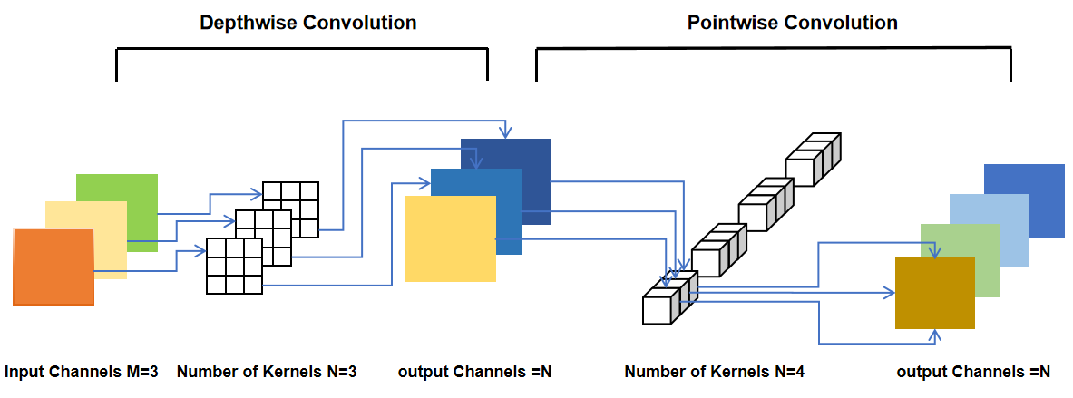
Figure 1. The process of Depthwise Separable Convolution.
Channel-separated convolution refers to the characteristic of depth-separable convolutional networks. Specifically, the network first performs spatial convolution for each channel (depth), generates a series of convolutional results, and then stitches these results together. The final feature map is then generated by the depth-separable convolutional network by applying channel convolution on the joining result using a unit convolution kernel.
The deep separable convolutional network offers a reduction in computational demand and parameter count when contrasted with its traditional convolutional neural network counterpart. The difference in the parameter counts and computational effort between the standard convolution (SC) and the deep separable convolution (DSC) is reflected in Table 2.
Table 2. Parameter counts and computational effort required for standard and depth-separable convolution. | |||
Standard Convolution | Deep Separable Convolution | ||
Parameter Counts | Computational Effort | Parameter Counts | Computational Effort |
\( {D_{K}}×{D_{K}}×M×N \) | \( {D_{K}}×{D_{K}}×M×N×H×W \) | \( {D_{K}}×{D_{K}}×M+{D_{K}}×N \) | \( {D_{K}}×{D_{K}}×M×H×W+{D_{K}}×N×H×W \) |
\( {D_{K}} \) represents the size of the convolutional kernel.
\( M \) stands for the number of input channels.
\( N \) represents the number of output channels.
\( H \) and \( W \) stand for the height and width of the input feature map respectively.
The ratio of the number of parameters and computational cost between SC and DSC:
\( \frac{Parameter Counts (SC)}{Parameter Counts (DSC)}=\frac{Computational Effort (SC)}{Computational Effort (DSC)}=\frac{1}{N}+\frac{1}{D_{K}^{2}}\ \ \ (1) \)
3.1.2. Convolutional Block Attention Module
By successively merging the two sub-modules of Channel Attention and Spatial Attention, the Convolutional Block Attention Module (CBAM) [9] is a widely-applied attentional mechanism that allows the model to concentrate more on important aspects in the image (Figure 2 and Figure 3).
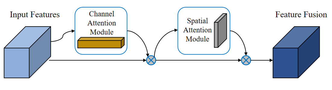
Figure 2. CBAM module flowchart.
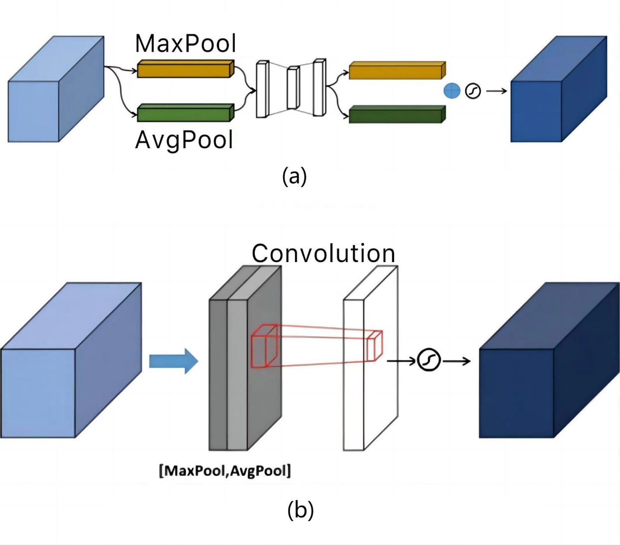
Figure 3. CBAM is composed of: (a) A channel attention module; (b) A spatial attention module.
To focus on the channel dimension, the feature matrix is initially inputted into the Channel Attention Module (CAM). Within this module, the feature maps undergo both global average pooling and global max pooling. These processes generate descriptors for the average-pooled features and the max-pooled features, respectively. And then MLP generates the channel attention and multiplies such attention weight values with the input feature matrix.
Following the channel attention mechanism, the feature matrix is fed into the Spatial Attention Module (SAM) to calculate attention in the spatial dimension. Additionally, along the channel axis, average pooling and maximum pooling operations are conducted to produce two two-dimensional mappings. After the two feature maps are stacked and run through a convolutional layer, the activation function finally produces the spatial attention map. To create a predicted feature map that is weighted in multiple dimensions of space and channel, the attention weight value is ultimately multiplied by the feature matrix with channel attention applied.
3.1.3. The Structure of DSConv-CBAM Model
In order to construct a model with a smaller number of parameters, less complexity, and superior feature extraction performance, this research proposed a network model based on depth-separable convolution and CBAM attention mechanism (DSConv-CBAM model). This innovative approach leverages the efficiency of depthwise separable convolution combined with the powerful feature focusing abilities of the CBAM (Figure 4).
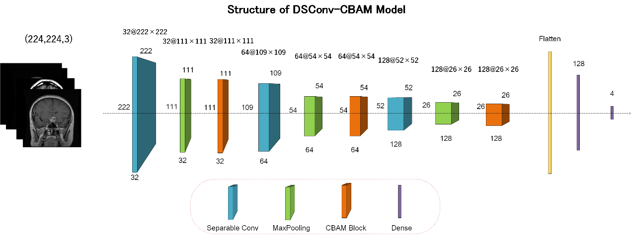
Figure 4. The structure of DSConv-CBAM model.
First, the input image passes through the first layer of SeparableConv2D using 32×3×3 convolution kernels for depth separable convolution to initially learn the local features of the MRI image. To reduce the size of the feature maps, MaxPooling operation is performed on the feature maps after depth-separable convolution, using a 2×2 pooling window. A CBAM attention module is introduced to refine the feature map with 32 input channels, a downscaling ratio of 16, and spatial attention using a 5×5 convolutional kernel.
For further feature abstraction, more complex features continue to be extracted using 64×3×3 convolutional kernels via SeparableConv2D and MaxPooling, subsequently following a CBAM module for feature refinement. Repeating the basic structure again, using the SeparableConv2D layer with 128 convolutional kernels, continued to reduce the feature map size through maximum pooling and used the CBAM module to further focus on key features.
The Flatten layer is utilized to bridge the convolution operation and the fully-connected operation to flatten the multidimensional output into one dimension. In order for the model to learn the images and labels, the model contains two fully connected layers. The first one has 128 neurons and the second one is the output layer with 4 neurons for outputting 4 classification results.
3.2. Multilayer Perceptron(MLP)
Multilayer perceptron is an artificial neural network (ANN) which contains an input layer, multiple hidden layers, and an output layer. Each layer is fully connected to the next layer, and each node except the input node carries a nonlinear activation function. The input data is forward propagated, the data is gradually propagated to the output layer, and the loss function is back-propagated to the first layer and the weights are updated. The structure of the MLP used in this research is shown in Figure 5.
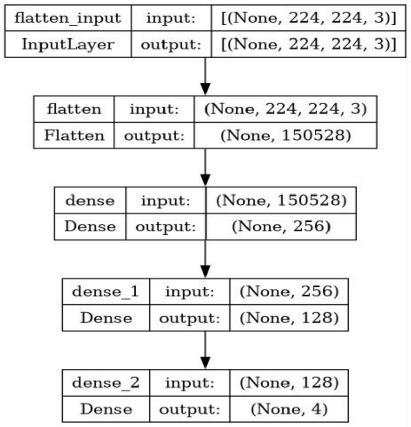
Figure 5. The structure of the MLP model.
3.3. Transfer Learning with Pre-trained MobileNetV2
Transfer learning is a method of using knowledge learned in one domain to apply it to another related domain. ImageNet is a widely used large-scale image dataset for training deep convolutional neural network models. In this study, we adopt the parameter transfer approach, utilizing the MobileNetV2 model pretrained on ImageNet, retaining all layers except for the final fully connected layer, and freezing the pretrained parameters. Additionally, we incorporated a global average pooling layer, a fully connected layer with 128 neurons, and a final output layer with 4 neurons.
3.4. Hyperparameter Settings
To train different models and compare the results, we set uniform hyperparameters before training. Specifically, we used Adam as the optimizer. The learning rate was 0.001, beta_ 1 parameter was 0.9, and beta_2 parameter was set as 0.99. ReLU was used as the activation function for the model, and the cross-entropy loss function was employed. Each model was trained for 35 iterations with a batch size of 64.
3.5. Evaluation Metrics
To evaluate the classification performance of different models, this study employed accuracy, precision, recall, F1 score, specificity, and AUC as evaluation metrics. The formulas for these metrics are as follows:
\( Accuracy=\frac{TP+TN}{Total}\ \ \ (2) \)
\( Precision=\frac{TP}{TP+FP}\ \ \ (3) \)
\( Recall=\frac{TP}{TP+FN}\ \ \ (4) \)
\( F1 Score=2×\frac{Precision×Recall}{Precision+Recall}\ \ \ (5) \)
\( Specificity=\frac{TN}{TN+FP}\ \ \ (6) \)
TP stands for true positives, which refers to the number of positive cases that the model accurately predicts as positive. True negatives (TN) refer to the accurate prediction of negative instances as negative by the model. FP stands for false positives, which refers to the count of negative cases that the model mistakenly predicts as positive. False negatives (FN) refer to the cases where the model wrongly predicts positive instances as negative.
4. Result and discussion
4.1. Training process
Figure 6 shows the validation accuracy curves of the model training process for the MLP model, the transfer learning MoblieNetV2 model and the self-constructed DSConv-CBAM model. From the curves, it can be seen that the transfer learning strategy can obtain a significantly higher initial accuracy with the fastest convergence speed compared to the additional two models trained from scratch, with convergence accomplished at about 10 epochs. On the other hand, the two models trained from scratch, the MLP and the DSConv-CBAM model, both have noticeably lower initial accuracies than the transfer learning model while converging at a significantly slower rate, completing convergence at about 20 and 15 epochs, respectively. On the other hand, the MLP experiences greater fluctuations during training and is more challenging to converge compared to the other two convolutional neural network models. Meanwhile, the DSConv-CBAM model's loss and accuracy curves are smoother than those of MobileV2.
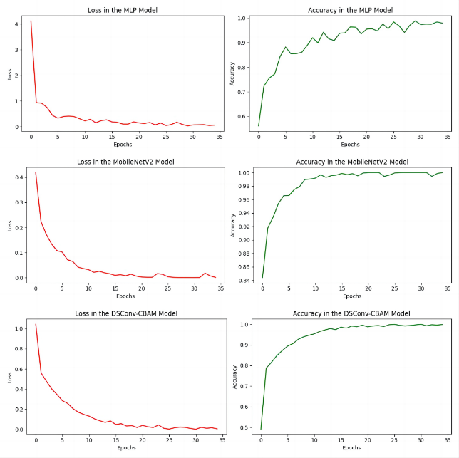
Figure 6. The loss and accuracy curves of different models.
4.2. Testing results
Table 3 presents the evaluation outcomes for three models. All the three models exhibit excellent recall when confronted with MRI medical images of pituitary tumors and no tumors, obtaining 97.67%, 98.67% and 99.67% recall for pituitary tumor cases and 100.00%, 99.75% and 100.00% recall for no tumor cases, respectively. All three models showed excellent ability in not to miss report pituitary tumors and no tumor cases. However, the MLP model demonstrated a mere 89% accuracy, with the lowest weighted average across other metrics, particularly notable in its recall for the Meningioma category at only 68%. This indicates a significant rate of missed diagnoses for the meningioma class.
In addition, the DSConv-CBAM model improves precision by 3.67% in the confrontation of MRI medical images of meningiomas and recall by 3.00% in the confrontation of MRI medical images of gliomas compared to the transfer learning MoblieNetV2 model.
To conclude, the DSConv-CBAM model outperforms the pretrained MobileNetV2 in overall accuracy and metrics. This showcases the superior performance of the DSConv-CBAM model.
Table 3. Test results of different models. | |||||||
Model | Classes | Precision | Recall | F1-Score | Specificity | Kappa | Accuracy |
MLP | Pituitary | 0.96 | 0.98 | 0.97 | 0.99 | 0.86 | 0.89 |
No tumor | 0.89 | 1.00 | 0.94 | 1.00 | |||
Meningioma | 0.89 | 0.68 | 0.77 | 0.91 | |||
Glioma | 0.84 | 0.89 | 0.86 | 0.97 | |||
Average | 0.90 | 0.89 | 0.89 | 0.97 | |||
MobileNetV2 | Pituitary | 0.97 | 0.99 | 0.98 | 1.00 | 0.96 | 0.97 |
No tumor | 1.00 | 1.00 | 1.00 | 1.00 | |||
Meningioma | 0.91 | 0.97 | 0.94 | 0.99 | |||
Glioma | 0.99 | 0.91 | 0.94 | 0.97 | |||
Average | 0.97 | 0.97 | 0.97 | 0.99 | |||
DSConv-CBAM | Pituitary | 0.98 | 1.00 | 0.99 | 1.00 | 0.97 | 0.97 |
No tumor | 0.99 | 1.00 | 1.00 | 1.00 | |||
Meningioma | 0.94 | 0.95 | 0.95 | 0.99 | |||
Glioma | 0.97 | 0.94 | 0.95 | 0.98 | |||
Average | 0.97 | 0.97 | 0.97 | 0.99 | |||
4.3. Confusion Matrix
This study presents the confusion matrices of three models, as shown in Figure 7. In the confusion matrices, the diagonal line stretching from the top-left to the bottom-right indicates the count of correct predictions for each category. The more numbers there are on the diagonal of the confusion matrix, the more accurate the model predictions are and the better the performance.
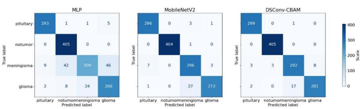
Figure 7. Confusion matrices of different models.
4.4. Discussion
In this research, a convolutional neural network model, DSConv-CBAM, combining deeply separable convolution and attentional mechanisms, was constructed for a brain tumor MRI medical image classification task.
Brain Tumor MRI Dataset [7], a freely available public dataset from Kaggle consisting of 5712 images for training and 1311 images for testing, was used to evaluate the performance of three types of models, the multilayer perceptron MLP, the transfer learning model MobileNetV2, and the DSConv-CBAM model, respectively, on the task of classifying MRI medical images of brain tumors, and to compute various evaluation metrics in terms of precision, recall, F1-score, specifity, kappa, and accuracy. According to the obtained results, the self-constructed model DSConv-CBAM achieved the highest accuracy in MRI tumor classification when confronted with this dataset, and the DSConv-CBAM model, the transfer learning model MobileNetV2, and MLP models achieved an accuracy of 97.41%, 96.72%, and 89.47%, respectively. Table 3 demonstrated the detailed evaluation scores of the three models on brain tumor MRI medical image classification, and despite the slightly lower scores in the individual subthemes targeting different types of tumors, the comprehensive ability of the self-constructed DSConv-CBAM model is still significantly better than the other models.
However, the test results also revealed some of the issues. All the models in this research, including the proposed DSConv-CBAM model, suffer from overfitting problems when facing small datasets. Due to the relatively minor size of the dataset, the models were over-matched to the current dataset after training, such that their performance showed significant degradation in the face of other data or while performing prediction, resulting in poor generalization ability of the models. The size of medical image datasets is usually very limited, while the medical image data used for model training usually demands manual feature extraction by human experts, which is limited by their accumulated level of expertise, time, and effort. Meanwhile, as a black-box model, the internal operation principle of the convolutional neural network model is usually complicated to elucidate, although it can classify and judge the medical image data for the reference of human experts, it cannot provide the basis of judgment for the human experts, which restricts the auxiliary ability of the human experts by its low interpretability.
How to apply other advanced data preprocessing methods, including data enhancement, image segmentation, to avoid the overfitting problem while further improving the generalization ability of the model and its computational efficiency to adapt to its application environment will be the direction of subsequent research. It is expected that the model can be applied to other tumor types like lung cancer, liver cancer, pancreatic cancer, as well as other medical images like PEI, x-ray, ultrasound images, and so on. It is hoped that as the size of the medical image database will continue to expand and the model algorithms will continue to be iteratively improved, in the future it will be possible to build a comprehensive system to help reduce the burden of assisted judgment of human experts working in the field of medicine.
5. Conclusion
This study presents the development of a new convolutional neural network model, DSConv-CBAM, specifically designed to improve the precision and efficiency of classifying brain tumour MRI images.By integrating depth-separable convolution with an attention mechanism, the model effectively balances performance with a reduced number of parameters, which is particularly beneficial for medical environments with limited computational resources. The model was rigorously evaluated against classical MLP and MobileNetV2 models, demonstrating superior accuracy in classifying gliomas, meningiomas, pituitary tumors, and non-tumors.
The DSConv-CBAM model's innovative architecture, which includes a depth-wise separable convolution layer and a CBAM module, allows for more efficient feature extraction and focus on significant image features, leading to an average classification accuracy of 97.41%. Despite the model's high performance on the dataset, challenges such as overfitting due to the dataset's limited size were noted, indicating the need for advanced data preprocessing techniques to improve generalization.
The study's findings suggested that the DSConv-CBAM model could serve as a valuable tool in medical diagnostics, potentially aiding healthcare professionals in making more informed decisions regarding brain tumor treatments. Future work will explore the model's applicability to other tumor types and medical imaging modalities, with the ultimate goal of creating a comprehensive system to assist medical experts in their diagnostic efforts.
Authors Contribution
All the authors contributed equally and their names were listed in alphabetical order.
References
[1]. Ferlay J, Colombet M, Soerjomataram I, et al 2021 Cancer statistics for the year 2020: An overview Int. J. Cancer. 149 778–9
[2]. Mabray M C, Barajas R F and Cha S 2015 Modern brain tumor imaging Brain Tumor Res. Treat. 3 8–23
[3]. Babu Vimala B, Srinivasan S, Mathivanan S K et al 2023 Detection and classification of brain tumor using hybrid deep learning models Sci. Rep. 13 23029
[4]. Martini M L and Oermann E K 2020 Intraoperative brain tumour identification with deep learning Nat. Rev. Clin. Oncol. 17 200–1
[5]. Choudhury C L, Mahanty C, Kumar R, Mishra B K. 2020 Brain tumor detection and classification using convolutional neural network and deep neural network. In Proceedings of the 2020 International Conference on Computer Science, Engineering and Applications (ICCSEA) pp 1–4
[6]. Khaliki M Z and Başarslan M S. 2024 Brain tumor detection from images and comparison with transfer learning methods and 3-layer CNN Sci. Rep. 14 2664
[7]. Nickparvar, M 2021 Brain Tumor MRI Dataset, Version 1.0. Retrieved March, 2024 from https://doi.org/10.34740/KAGGLE/DSV/2645886
[8]. Howard A G, Zhu M, Chen B, et al. 2017 MobileNets: Efficient convolutional neural networks for mobile vision applications Preprint arXiv:1704.04861.
[9]. Woo S, Park J, Lee J Y, et al. 2018 Cbam: Convolutional block attention module. In Proceedings of the European conference on computer vision (ECCV) pp 3-19
Cite this article
Chen,W.;Sun,P.;Zhang,Y. (2024). A brain tumor diagnosis approach based on deep separable convolutional networks and attention mechanisms. Applied and Computational Engineering,67,60-69.
Data availability
The datasets used and/or analyzed during the current study will be available from the authors upon reasonable request.
Disclaimer/Publisher's Note
The statements, opinions and data contained in all publications are solely those of the individual author(s) and contributor(s) and not of EWA Publishing and/or the editor(s). EWA Publishing and/or the editor(s) disclaim responsibility for any injury to people or property resulting from any ideas, methods, instructions or products referred to in the content.
About volume
Volume title: Proceedings of the 2nd International Conference on Software Engineering and Machine Learning
© 2024 by the author(s). Licensee EWA Publishing, Oxford, UK. This article is an open access article distributed under the terms and
conditions of the Creative Commons Attribution (CC BY) license. Authors who
publish this series agree to the following terms:
1. Authors retain copyright and grant the series right of first publication with the work simultaneously licensed under a Creative Commons
Attribution License that allows others to share the work with an acknowledgment of the work's authorship and initial publication in this
series.
2. Authors are able to enter into separate, additional contractual arrangements for the non-exclusive distribution of the series's published
version of the work (e.g., post it to an institutional repository or publish it in a book), with an acknowledgment of its initial
publication in this series.
3. Authors are permitted and encouraged to post their work online (e.g., in institutional repositories or on their website) prior to and
during the submission process, as it can lead to productive exchanges, as well as earlier and greater citation of published work (See
Open access policy for details).
References
[1]. Ferlay J, Colombet M, Soerjomataram I, et al 2021 Cancer statistics for the year 2020: An overview Int. J. Cancer. 149 778–9
[2]. Mabray M C, Barajas R F and Cha S 2015 Modern brain tumor imaging Brain Tumor Res. Treat. 3 8–23
[3]. Babu Vimala B, Srinivasan S, Mathivanan S K et al 2023 Detection and classification of brain tumor using hybrid deep learning models Sci. Rep. 13 23029
[4]. Martini M L and Oermann E K 2020 Intraoperative brain tumour identification with deep learning Nat. Rev. Clin. Oncol. 17 200–1
[5]. Choudhury C L, Mahanty C, Kumar R, Mishra B K. 2020 Brain tumor detection and classification using convolutional neural network and deep neural network. In Proceedings of the 2020 International Conference on Computer Science, Engineering and Applications (ICCSEA) pp 1–4
[6]. Khaliki M Z and Başarslan M S. 2024 Brain tumor detection from images and comparison with transfer learning methods and 3-layer CNN Sci. Rep. 14 2664
[7]. Nickparvar, M 2021 Brain Tumor MRI Dataset, Version 1.0. Retrieved March, 2024 from https://doi.org/10.34740/KAGGLE/DSV/2645886
[8]. Howard A G, Zhu M, Chen B, et al. 2017 MobileNets: Efficient convolutional neural networks for mobile vision applications Preprint arXiv:1704.04861.
[9]. Woo S, Park J, Lee J Y, et al. 2018 Cbam: Convolutional block attention module. In Proceedings of the European conference on computer vision (ECCV) pp 3-19