1.Introduction

The real estate industry is crucial to China's economy, serving as a pillar industry and playing a pioneering role during rapid urbanization. After the Reform and Opening-up, China transitioned from a rural society to an urbanized one, with housing demand outpacing supply. From 1998 to 2020, the average price of commercial housing nationwide increased from 20k yuan to 100k yuan. Before COVID-19, the real estate market significantly boosted economic growth, with development investment contributing over 10% to economic growth for many years [1].

The COVID-19 epidemic marked a turning point, causing a shock to real estate demand and construction. The suspension of property sales increased capital chain tensions, leaving projects abandoned. Real estate share prices and property values were negatively affected, and the growth rate of national real estate development investment declined significantly [2]. Figure 1 shows the trend, dominated by the continuous fall, of the national real estate climate index from early 2021 to the end of 2023 [3][4]. In August 2020, the "Three Red Lines" financial regulations were introduced to govern corporate debt financing, impacting the high-leverage, high-growth model. Despite evidence of the immediate negative impacts of the policies, some researchers believe these policies will benefit long-term development [5][6][7].

Given these challenges, investigating real estate productivity is essential to provide deeper insights and promote high-quality development. Data Envelopment Analysis (DEA) measures the efficiency of real estate companies. Previous studies have applied DEA in various markets, demonstrating its utility in assessing efficiency [8][9][10][11]. However, the DEA frontier is very sensitive to the presence of outliers and statistical noise [12], the efficient frontier derived from DEA may be warped if the data are contaminated by statistical noise. Besides, DEA can hardly be used to predict the performance of other decision-making units [13]. Neural Networks (NN) address these limitations by solving non-linear problems and creating a smooth, continuous frontier [14]. Integrating DEA with NN improves robustness, Patel (2015) [15] used NN to smooth DEA's frontier, providing a more accurate evaluation of DMUs.

Few studies have applied neural networks to analyze the efficiency of China's real estate enterprises, this paper aims to provide a review and insight into the operating efficiency of 87 listed real estate development companies in China in 2023. The following work in Figure 2 is done in the paper to establish an enhanced frontier to evaluate the efficiency of the selected companies in 2023. Initially a super-efficiency SBM is performed to get the original evaluation of companies, and then a BPNN is trained to fit an enhanced frontier which is eventually used to re-evaluate the efficiency. Compared to the original frontier, the enhanced frontier provides a more robust evaluation of efficiency by capturing the slacks omitted by the super-efficiency SBM DEA.

Figure 1. National Real Estate Climate Index (From NBS China)

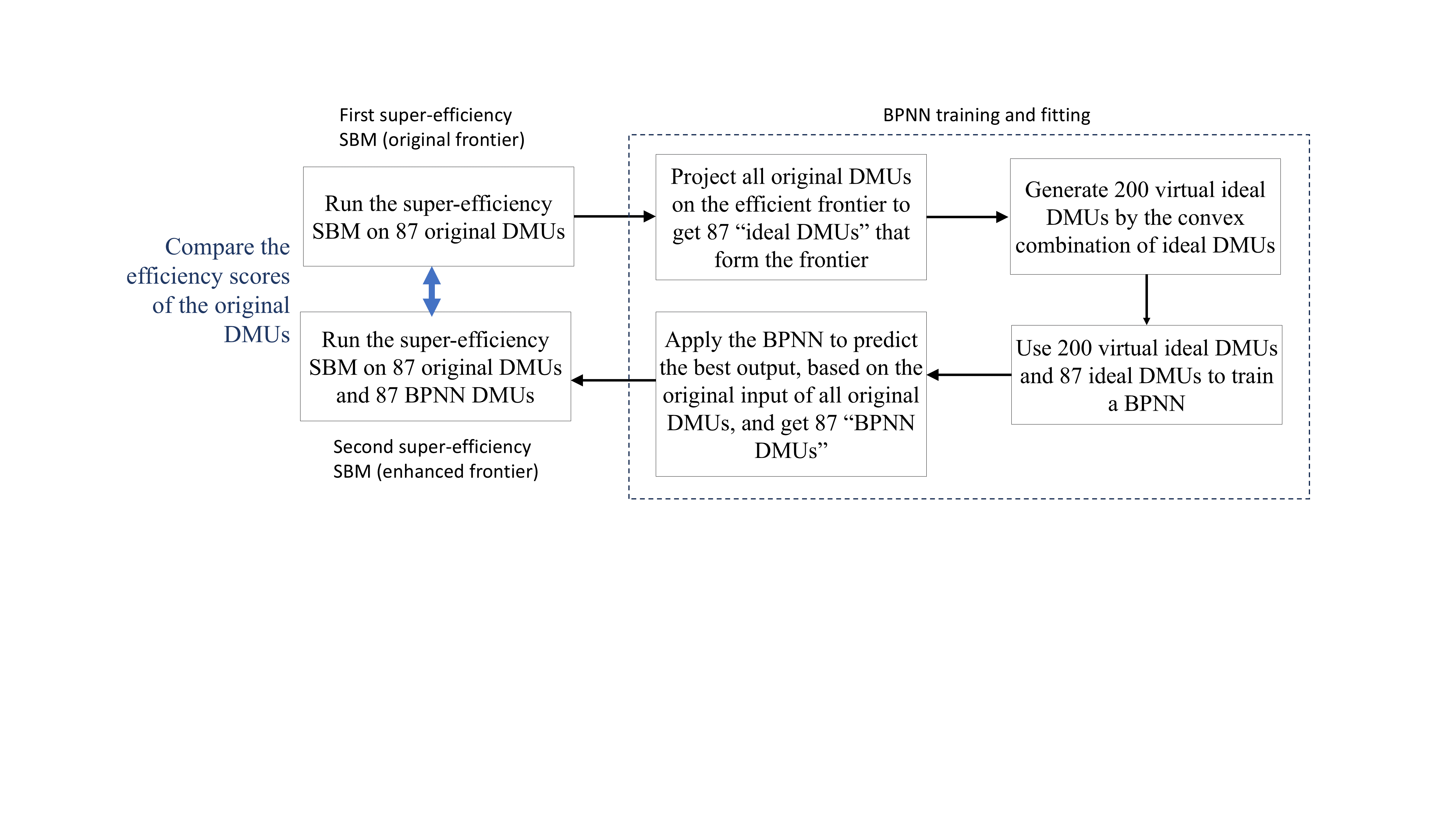
Figure 2. The Construction Process of “Neural Network Frontier”

2.Methodology

2.1.Data envelopment analysis (DEA)

2.1.1.CCR model. The CCR model is a basic DEA model assuming constant returns to scale (CRS) and is radial in nature, as it aims to achieve the greatest proportional reduction in all inputs or expansion in all outputs. The efficiency score of a DMU is derived from how much its inputs can be contracted or outputs expanded proportionately.

The CCR model has two orientations: input- and output-oriented. The orientation corresponds to whether the goal is to reduce excess inputs or expand shortfalls in outputs to move the inefficient unit to the frontier. For instance, in an input reduction model, the greatest percentage reduction in all inputs is sought. The red arrow in Figure 3 illustrates radial improvement for a 2-input, 1-output case. DMU B is diagonally moved to DMU E which lies on the frontier.

To assume there are n DMUs, namely\( {DMU_{j}} (j=1, 2, …, n) \), each DMU includes m input variables\( {X_{j}}={({x_{1j}}, {x_{2j}},…, {x_{mj}})^{T}} \), s output variables\( {Y_{j}}={({y_{1j}}, {y_{2j}}, …, {y_{qj}})^{T}} \), then a output-oriented CCR model of\( {DMU_{j0}} \)is provided by this linear programming (LP):

•\( \underset{ϕ, λ}{max}{ϕ}{ } \)

\( s.t.\begin{cases}\sum {X_{j}}{λ_{j}}≤{X_{0}} \\ \sum Yj{λ_{j}}≥{ϕY_{0}} \\ {λ_{j}}≥0 (∀j)\end{cases}\ \ \ (1) \)

in which\( ({X_{0}},{Y_{0}}) \)is the input and output of\( {DMU_{j0}} \),\( {λ_{j}} \)denotes the intensity of\( {DMU_{j}} \)when the linear frontier of efficient DMUs is formed, therefore\( \sum {X_{j}}{λ_{j}} \)and\( \sum {Y_{j}}{λ_{j}} \)plot the efficient frontier. This formula means that within the production possibility set\( T \), while maintaining output\( {X_{0}} \)​ without increase, the input vector\( {Y_{0}} \)​ is maximized proportionally to\( ϕ{Y_{0}} \)​. If the output cannot be enlarged, namely the maximum value of\( ϕ \)is 1, the evaluated DMU is considered an efficient unit; otherwise, it is relatively inefficient.

2.1.2.Super-efficiency SBM. The CCR model is unable to fully capture the impact of slackness on efficiency. In Figure 3, DMU B is more efficient than DMU E', as DMU B's input2 productivity is higher than that of DMU E' while controlling for input1 productivity. However, both DMUs are identified as efficient by the CCR model. The slack-based measure (SBM) addresses this issue by introducing "slacks", which quantify the inefficiencies by indicating the degree to which inputs can be decreased or outputs can be increased while still maintaining the current level of outputs and inputs, respectively. In SBM, input and output factors do not need to change proportionally, but need to eliminate the slacks. The movement from DMU E' to B which is plotted as a blue arrow in Figure 3 represents a slack improvement, recognizing B as more efficient than E', and E is the least efficient in this 3 DMUs.

When many DMUs are found efficient in a DEA model, the relative efficiency comparison fails as all efficient DMUs score 1. To address this, super-efficiency DEA models can be used. In a super-efficiency model, the DMU being evaluated is excluded from its own comparison set, removing the upper limit of 1 on efficiency scores and allowing scores greater than 1, which can rank efficient units. An output-oriented super-efficiency SBM with constant returns to scale is given by:

•\( \underset{λ, {s^{-}}, {s^{+}}}{max}{ρ=1/(1+\frac{1}{q}\sum _{r=1}^{q}\frac{s_{r}^{+}}{{y_{io}}})}{ } \)

\( s.t.\begin{cases}{X_{0}}≥+{s^{-}} \\ {Y_{0}}≤-{s^{+}} \\ {λ_{j}}≥ 0 (∀j), {s^{-}}≥0, {s^{+}}≥0\end{cases}\ \ \ (2) \)

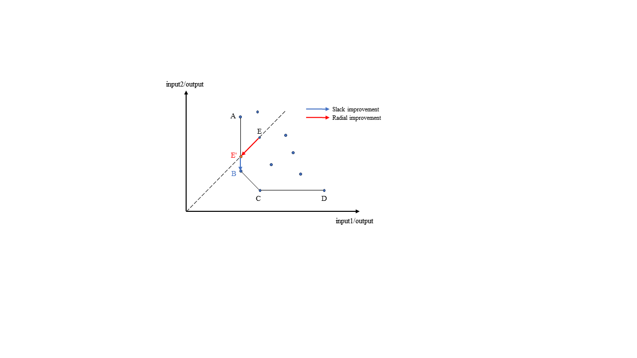
Figure 3. Efficient Frontier and Efficiency Improvement in DEA

2.2.Neural network

The neural network is a machine learning algorithm composed of interconnected processing units arranged into layers [16]. Each unit has multiple inputs, each with an associated weight. The unit performs a weighted summation of the inputs, applies a transfer function, and transmits the output to the next layer. A classic model is the backpropagation neural network (BPNN), a multi-layer forward neural network trained using the error backpropagation algorithm. BPNN can solve non-linear problems that simple perceptions cannot. It consists of three layers: input, hidden, and output. Using the gradient descent algorithm, it minimizes the square of the error between the actual and expected outputs.

In this paper, a BPNN with 3 layers and 128 neurons in each layer was trained. The network used 3 input variables as features and 2 output variables as labels, with ReLU for the hidden layers and a linear activation function for the output layer. The architecture of the BPNN is shown in Figure 4.

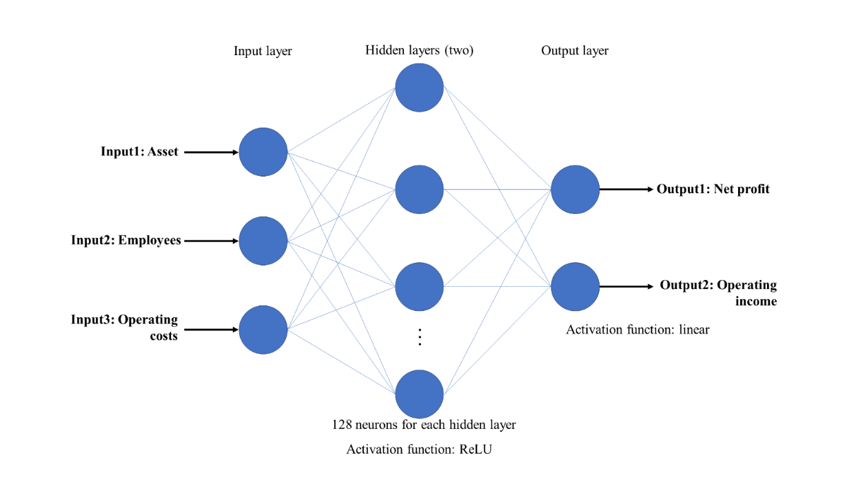
Figure 4. The architecture of BPNN

3.Data selection and descriptive statistics

Data from 87 real estate development companies listed on the Shanghai Stock Exchange or Shenzhen Stock Exchange in 2023 is selected from CSMAR. Table 1 shows the variable selection and denotation. Figure 5 plots the distribution of these variables. These variables are relatively concentrated in most companies, with a few larger-scale companies. The number of companies with positive net profit is roughly equal to the number of companies with negative net profit.

Table 1. The Selected Variables for DEA

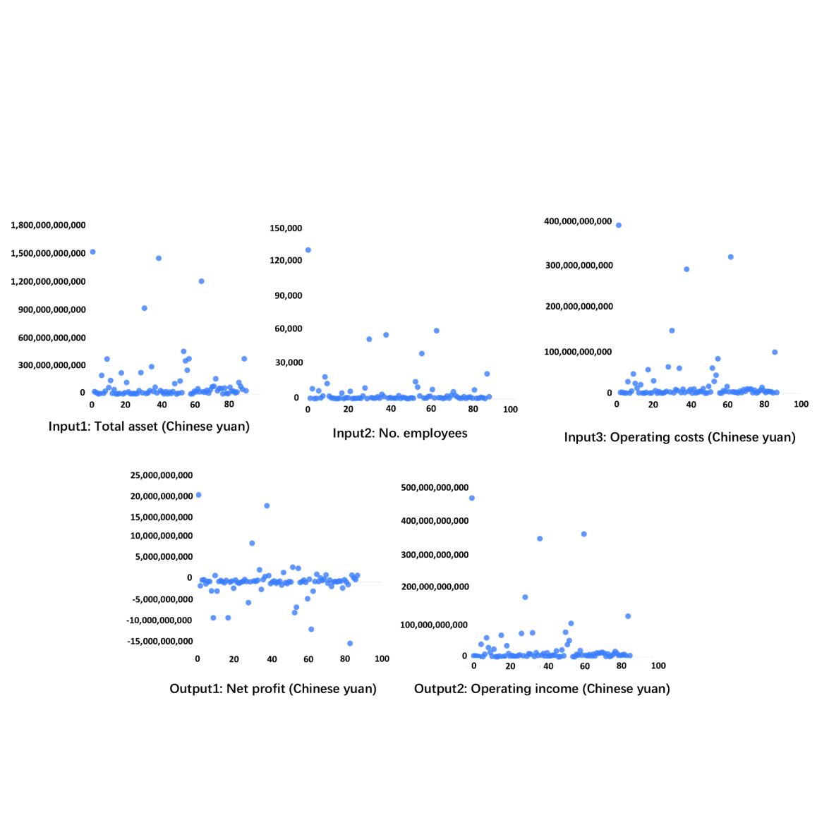
Figure 5. Distribution of the Selected Variables

4.Empirical results analysis

4.1.Original measure of efficiency: Super Efficiency SBM-DEA

The output-oriented super-efficiency SBM DEA is performed on Python to evaluate the operating efficiency of these 87 companies as “original DMUs”. 3 input variables and 2 output variables listed in Table 1are used. To perform the DEA, all variables are Min-Max normalized to scale the variables of this dataset between 0 and 1 for large differences in the original magnitudes which makes the model solution biased or infeasible. A negative net profit is assigned as 0.01. In Tabel 2, the first column shows the 6-digit codes for Shanghai and Shenzhen A-shares assigned to these companies listed on the Shanghai Stock Exchange and the Shenzhen Stock Exchange. The original efficiency scores of all DMUs are listed in the second column of Table 2 in descending order.

Table 2. The Efficiency Evaluation Results

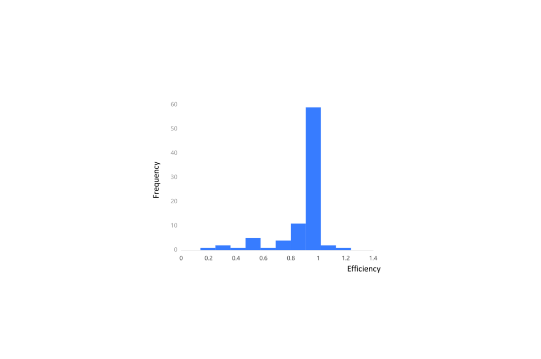
Figure 6. Frequency Distribution of Efficiency in the Original Evaluation

There are 13 efficient DMUs that have an efficiency of not less than 1. 73.5% of these companies have an efficiency higher than 0.9. It was found that most of the DMUs have efficiency scores concentrated between 0.8 and 1. Figure 6 shows that when the efficiency drops from 0.9 to 0.8, the number of DMUs decreases sharply. This evaluation suggests that the majority of the companies exhibit comparable operational efficiency, with little difference from the top-performing companies.

4.2.Revised measure of efficiency: using BPNN to enhance the frontier

Based on super-efficiency SBM DEA, I aim to determine more robust and realistic efficiency scores for DMUs. DEA models often provide exaggerated efficiency scores because efficiency is measured relative to available DMUs. A small proportion of efficient DMUs establishes a rough frontier, potentially overestimating DMU efficiency. Figure 7 illustrates a 2-input, 1-output SBM model with a non-smooth original frontier. X on this frontier is X', and vector XX' can be decomposed into two orthogonal slack vectors. In an output-oriented SBM model, a DMU’s efficiency is determined by its slacks; larger output slacks indicate lower efficiency

A non-smooth frontier can underestimate the distance between a DMU and the efficient frontier. If point R does not exist in Figure 7, DMUs A, Q, B, and C form the efficient frontier. When DMU R appears between points A and B, the frontier changes to ARBC. In reality, DMU R represents DMUs missing from the corpus due to a lack of observations and is not an extreme value. DMU R likely belongs to the production possibility set and can form a smoother frontier with points A, B, and C. The slack vectors decomposed from vector PR are larger than the original slack vectors, indicating the original frontier omitted some actual output slack, resulting in underestimated slack and overestimated efficiency for point P.

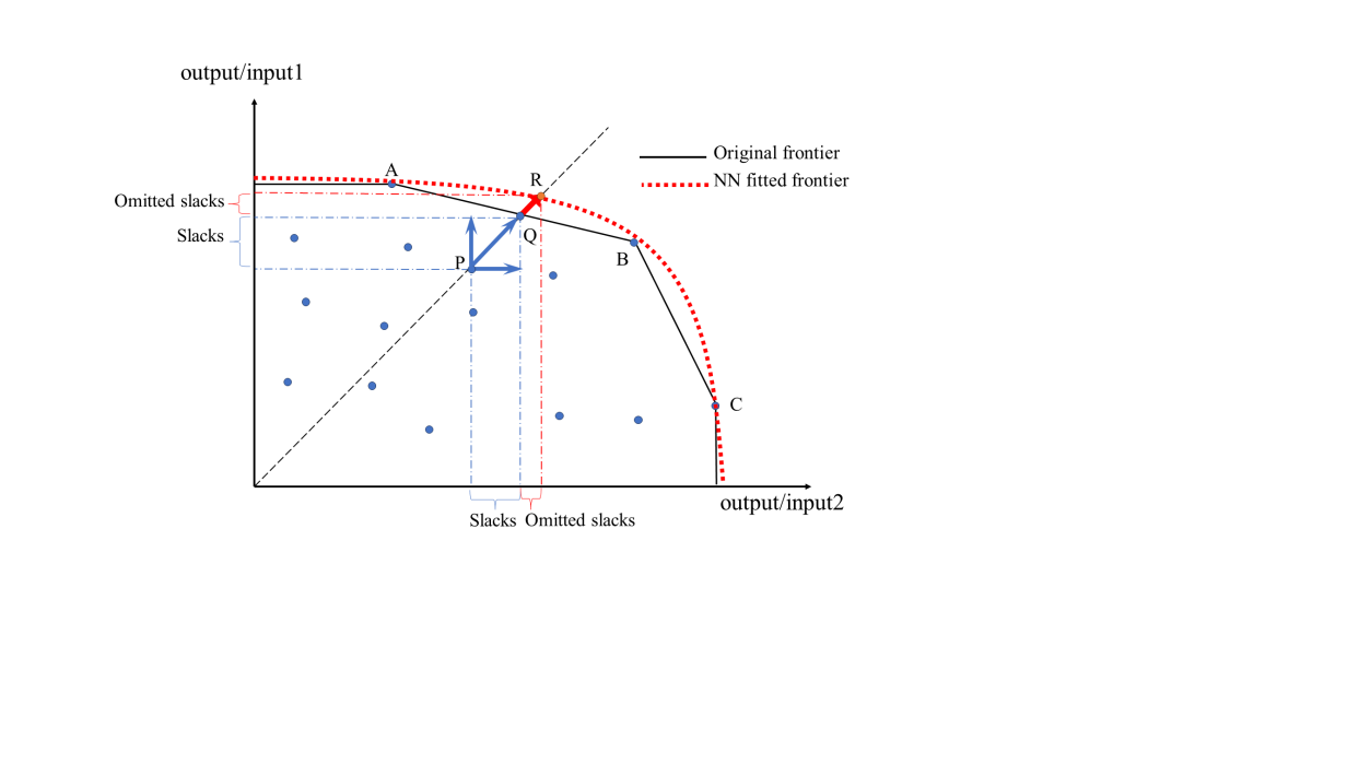
Figure 7. NN enhanced frontier adjusts the underestimated slacks and overestimated efficiency

Based on the above, I used a backpropagation neural network (BPNN) to simulate an enhanced frontier that is smoother by including as many potentially unobserved valid DMUs similar to R as possible in the corpus. This approach provides more robust efficiency estimates for the initial DMUs, addressing the common issue of SBM DEA underestimating slacks.

I firstly projected 87 original DMUs onto the original frontier by deducting slacks from the input variables and adding slacks to the output variables. This process created 87 “ideal DMUs” that accurately represent the original efficiency frontier. These ideal DMUs are all considered efficient. Next, I generated an additional 200 virtual ideal DMUs, each a convex linear combination of all 87 ideal DMUs, ensuring these virtual DMUs are also efficient. Using Python 3.12, I then trained a BPNN with the 87 ideal DMUs and the 200 virtual DMUs. The training used 3 input variables as features and 2 output variables as labels, employing 5-fold cross-validation and training the model for 500 epochs to ensure robustness. This BPNN model effectively learns the relationship between the input and output of efficient DMUs. The BPNN model was then used to predict the optimal outputs for the 87 original DMUs by using their input variables. The predicted best outputs, combined with the original inputs, formed a new set of 87 “fitted DMUs.” These fitted DMUs simulate the efficient but unobserved DMUs that might exist within the corpus. Finally, all original DMUs and fitted DMUs were applied in Super SBM-DEA. The fitted DMUs formed an enhanced frontier. The efficiency re-evaluation results are shown in the third column of Table 2.

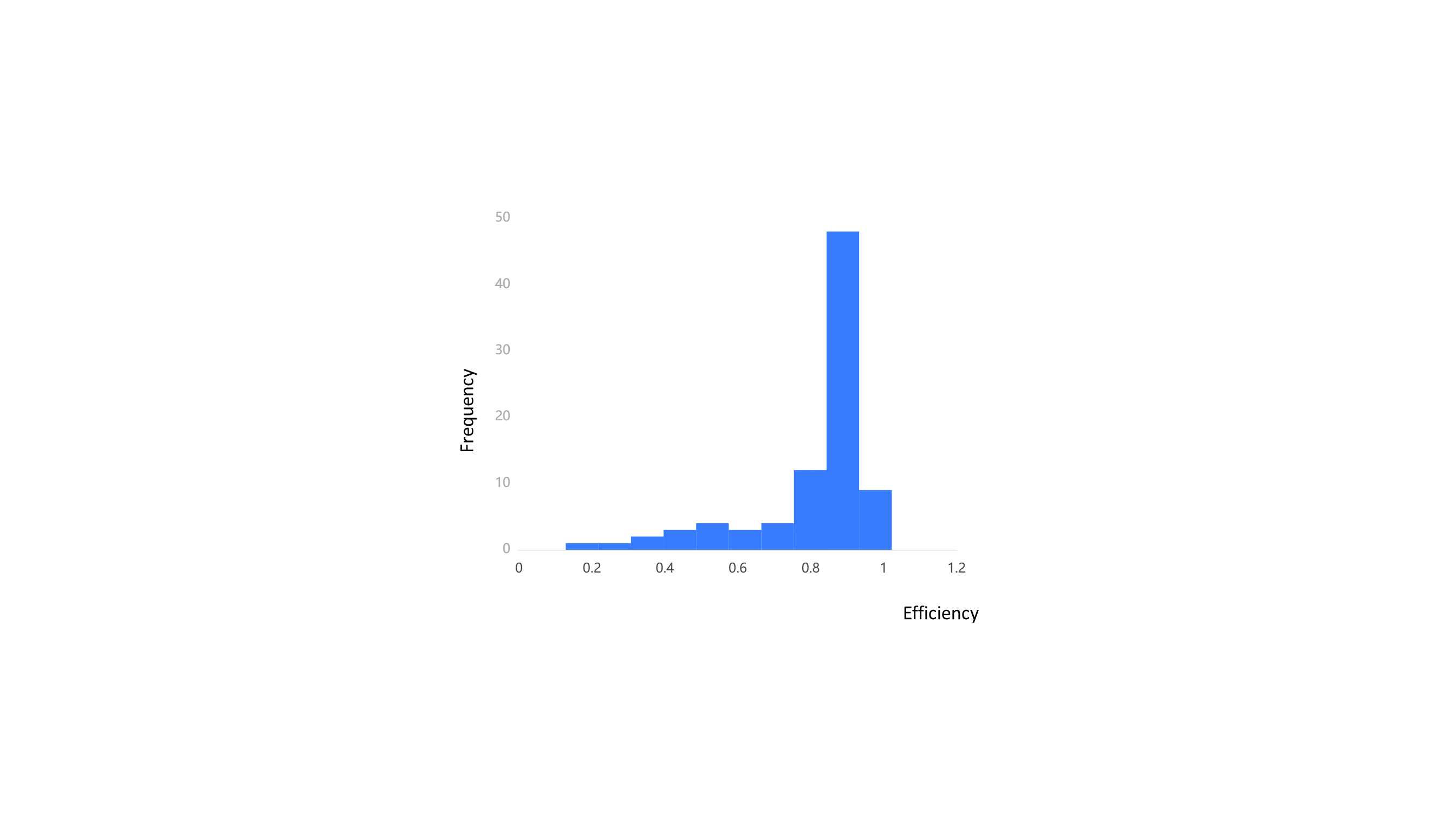
Figure 8. Frequency Distribution of Efficiency in the Adjusted Evaluation

After re-evaluating the efficiency of the original DMUs, it is clear that the re-evaluated efficiency scores for all companies dropped, with an average percentage decrease of 8.34%. The mean efficiency decreased by 8.2% compared to the original evaluation, and 47.13% of the companies have efficiency scores over 0.9. Compared to the initial efficiency distribution in Figure 8, Figure 6 indicates that the efficiency scores in the reevaluation are more dispersed, allowing for better differentiation of efficiency differences between companies. The goal of establishing an enhanced frontier using fitted DMUs to reduce the overestimation of the original DMUs' efficiency has been achieved. The original rough frontier is well enveloped by the enhanced, smoother, and expanded frontier. To further ensure the enhanced frontier's effectiveness, I additionally added the ideal DMUs obtained from the projection in step 1 into another calculation. The efficiency scores of the original DMUs did not change, and the average score of the ideal DMUs that construct the original frontier is 0.940, which is very close to the efficient level. This means the enhanced frontier does not excessively deviate from the original frontier, ensuring that the DMUs on the original frontier and the DMUs enveloped in the original frontier are not excessively underestimated. The re-evaluated efficiency is a robust adjustment to the original efficiency.

To verify the ability of the re-evaluated efficiency to accurately reflect the original efficiency, a regression analysis was conducted. This analysis aimed to determine the extent to which the re-evaluated efficiency can serve as a reliable proxy for the original efficiency scores. The results are shown in Table 3. The regression coefficient is significantly different from zero and close to one, with an R² value of 0.995. This indicates that the re-evaluated efficiency can serve as a reliable proxy for the original efficiency.

Table 3. Linear Regression Results of the Reevaluated Efficiency to The Original Efficiency

To identify which DMUs undergo the largest adjustments in the re-evaluation, I performed a multiple regression analysis of the percentage change in efficiency against the slack variables of the original DMUs from the first DEA calculation. The results are shown in Table 4. It can be observed that DMUs with larger slacks in total assets and number of employees, but smaller slacks in operating income in the initial DEA calculation are more likely to undergo significant adjustments in the reevaluation. This indicates that DMUs with larger input redundancies and smaller output shortfalls are more likely to undergo greater adjustments in the reevaluation. Those DMUs that achieved higher efficiency scores primarily due to underestimated output shortfalls will receive lower scores in the reevaluation. This aligns with the objective of the output-oriented model, which is to guide improvements in output.

Table 4. Linear Regression Results of Slacks to the Percentage of Efficiency Change

5.Conclusion

This paper examines 87 real estate development companies listed on the Shenzhen and Shanghai markets, analyzing their input and output data from 2023. Firstly, the paper employs the output-oriented super-efficiency SBM DEA method to evaluate the operational efficiency of the selected companies. It finds that the operational efficiency of most companies is above 0.8, with 73.5% of the companies having an operational efficiency greater than 0.9. To address the issue of overestimated DMU efficiency in the original model, this paper integrates the backpropagation neural network (BPNN) algorithm into the output-oriented super-efficiency SBM DEA method. By using this method, the study provides robust efficiency estimates for the selected companies. All companies' efficiency scores decreased compared to the original evaluation, with an average percentage decrease of 8.34%. The mean efficiency in the reevaluation decreased by 8.2% compared to the original evaluation, with 47.13% of the companies having an efficiency greater than 0.9. The overall decrease in efficiency scores after training an enhanced frontier with the BPNN and incorporating it into the efficiency evaluation aligns with the expectations for this "neural network frontier." The neural network frontier method does not excessively underestimate the efficiency of the companies and has good proxy capabilities for the original efficiency scores. The results of efficiency evaluation using the BPNN to establish an enhanced frontier are robust and effective. Additionally, the enhanced frontier significantly corrects the efficiency scores of companies with originally smaller output slacks, effectively identifying and assigning lower efficiency scores to those with underestimated output shortfalls. This combined super-efficiency SBM DEA and neural network efficiency evaluation method has the potential to be further applied to other output-oriented efficiency evaluation problems.

References

[1]. Ni, P., Ni, Z., Xu, H. (2023) Research on New Models and Construction of China's Real Estate Development. China Real Estate Finance, 06: 52–59.
[2]. National Bureau of Statistics of China. (2022) National Real Estate Development and Sales in 2021. https://www.stats.gov.cn/english/PressRelease/202201/t20220118_1826502.html
[3]. National Bureau of Statistics of China. (2023) National Real Estate Development and Sales in 2022. https://www.stats.gov.cn/english/PressRelease/202301/t20230118_1892298.html
[4]. National Bureau of Statistics of China. (2024) Investment in Real Estate Development in 2023. https://www.stats.gov.cn/english//PressRelease/202402/t20240201_1947107.html
[5]. Chen, Z., Gao, P., Liang, K. (2023) Impact of COVID-19 on China’s Real Estate Industry - An Empirical Study Based on the Stock Market. In: 2nd International Conference on Business and Policy Studies. Singapore. pp. 83.
[6]. Lin, A., Hale, T., Lockett, H. (2021) Half of China’s top developers crossed Beijing’s ‘red lines.’ Financial Times, 9.
[7]. Chu, X., Deng, Y., Tsang, D. (2023) Firm leverage and stock price crash risk: The Chinese real estate market and three-red-lines policy. J. Real Estate Finance Econ., 1–39.
[8]. Wong, W.P., Gholipour, H.F., Bazrafshan, E. (2012) How efficient are real estate and construction companies in Iran's close economy? Int. J. Strateg. Prop. Manag., 16(4): 392–413.
[9]. Chen, Q., Li, F. (2017) Empirical analysis on efficiency of listed real estate companies in China by DEA. iBusiness, 9(3): 49–59.
[10]. Zheng, X., Chau, K.W., Hui, E.C. (2011) Efficiency assessment of listed real estate companies: an empirical study of China. Int. J. Strateg. Prop. Manag., 15(2): 91–104.
[11]. Atta Mills, E.F.E., Baafi, M.A., Liu, F., Zeng, K. (2021) Dynamic operating efficiency and its determining factors of listed real‐estate companies in China: A hierarchical slack‐based DEA‐OLS approach. Int. J. Finance Econ., 26(3): 3352–3376.
[12]. Bauer, P.W. (1990) Recent developments in the econometric estimation of frontiers. J. Econom., 46(1-2): 39–56.
[13]. Wu, D.D., Yang, Z., Liang, L. (2006) Using DEA-neural network approach to evaluate branch efficiency of a large Canadian bank. Expert Syst. Appl., 31(1): 108–115.
[14]. Zhong, K., Wang, Y., Pei, J., Tang, S., Han, Z. (2021) Super efficiency SBM-DEA and neural network for performance evaluation. Inf. Process. Manag., 58(6): 102728.
[15]. Bose, A., Patel, G.N. (2015) “NeuralDEA”–A framework using Neural Network to re-evaluate DEA benchmarks. OPSearch, 52: 18–41.
[16]. Cane, V.R. (1967) Mathematical models for neural networks. In: Proceedings of the Fifth Berkeley Symposium on Mathematical Statistics and Probability. Berkeley. pp. 21–26.
Cite this article
Chen,W. (2024). Using super-efficiency slack-based measure data envelopment analysis with enhanced “neural network frontier” to evaluate the operating efficiency of Chinese-listed real estate companies. Applied and Computational Engineering,92,196-205.
Data availability
The datasets used and/or analyzed during the current study will be available from the authors upon reasonable request.
Disclaimer/Publisher's Note
The statements, opinions and data contained in all publications are solely those of the individual author(s) and contributor(s) and not of EWA Publishing and/or the editor(s). EWA Publishing and/or the editor(s) disclaim responsibility for any injury to people or property resulting from any ideas, methods, instructions or products referred to in the content.
About volume
Volume title: Proceedings of the 6th International Conference on Computing and Data Science
© 2024 by the author(s). Licensee EWA Publishing, Oxford, UK. This article is an open access article distributed under the terms and
conditions of the Creative Commons Attribution (CC BY) license. Authors who
publish this series agree to the following terms:
1. Authors retain copyright and grant the series right of first publication with the work simultaneously licensed under a Creative Commons
Attribution License that allows others to share the work with an acknowledgment of the work's authorship and initial publication in this
series.
2. Authors are able to enter into separate, additional contractual arrangements for the non-exclusive distribution of the series's published
version of the work (e.g., post it to an institutional repository or publish it in a book), with an acknowledgment of its initial
publication in this series.
3. Authors are permitted and encouraged to post their work online (e.g., in institutional repositories or on their website) prior to and
during the submission process, as it can lead to productive exchanges, as well as earlier and greater citation of published work (See
Open access policy for details).