1. Introduction

Sorting algorithms are very common in the research field for decades due to the need for sorting in all kinds of domains. Sorting algorithms have been used specifically for some sorting requirements, for example the computations for data processing, high-speed sorting[1], improving memory performance, and sorting using only one CPU. The algorithms create convenience for dealing with many complex problems.

As the ever-increasing computational power of parallel processing of parallel processing on many GPUs related to the processing system, many researches focus on how to use the calculation ability of those resources to do efficient sorting. However, not all of the domains of the calculation and the sorting application programming could make good use of the high throughput of these systems, so there is a desperate need for more creative and transformative methods to solve these shortages. In addition, with more serious and complex problems being solved by sorting algorithms, many common sorting algorithms have different applications in many fields and achieved effective results. This article will analyze the steps of all of the algorithms and list the applications of these algorithms. Additionally, a table will be provided to compare the time complexity (best, average, and worst) of these algorithms.

2. Sorting algorithm

2.1. Bubble sorting

By treating the sorting sequence from front to back, the value of the two adjacent elements are compared pairwise, if the reverse order is found, the exchange is made, so that the larger value of the element gradually moves from the front to back, as if the bubble under the water gradually rises.

Just as in Figure 1. Bubble sorting has some famous applications

It could be used in the successive-approximation-register ADC which contains a sample ,hold circuit, a capacitive array, a comparator, and a SAR control logic unit.

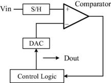
Figure 1. Structure of SAR ADC[1].

When it comes to the charge redistribution SAR DACs, the high accuracy of it needs the high matching of capacitors, which will result in a large chip area, then deteriorates the power consumption and sampling speed of ADC[2].In order to overcome the shortcomings, a calibration method can be used[3].

First, let n samples be arranged in an increasing order according to their values, this probability density function could be used to calculate the i-th order sample: fo,i(x)=n![F(x)]i-1[1-F(x)]n-1f(x)/(i-1)!(n-1)!

F(x) is the cumulative distribution function and the dF(x)=f(x)dx, x is the value of an ordered quantity, and according to the function FN(x)=1/(2Π)1/2*exp(-x2/2), and finally. could get Figure 2

.

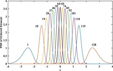
Figure 2. The ordered elements.

Combine the symmetrical elements to reduce offset and the elements are i-th and the (n-i+1)-th. This method could help rectify the mismatch of the unit capacitor in an ADC. When power is on, bubble sorting can be used to reorganize the capacitor binary structure to balance capacitors which are not matched. Figure 3 illustrates procedures of the calibration of eight units.

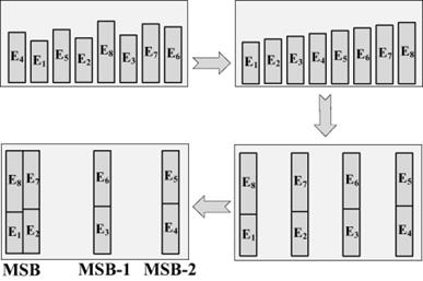
Figure 3. The process of calibration.

The reorganization could help ADC convert signals normally, and it could improve the efficiency of Artificial Free Dynamic Range and Signal-to-Noise-and-Distortion Ratio greatly.

2.2. Selection sorting

The characteristic of sorting selection is simple and direct. The specific operation is to select the smallest or largest element from the data elements that are not sorted, and then put it at the end of the sorting sequence until all the data elements to be sorted have been sorted. The selection sorting algorithm realizes sorting through selection and exchange, and the steps of their sorting are following:

First of all, select the smallest or the greatest element and exchange them with the data at first. And then, select the second smallest or largest element from the remaining n-1 data and swap it with the data in the second position. Next, repeat this process until the last two pieces of data are swapped. Finally, the original array is sorted from smallest to largest or from largest to smallest.

The time complexity of selecting sorting is O(n2). The selection sorting algorithm could be used in the visualization design. The most typical example is used in the Multimedia Development Life Cycle[4]. It may conclude six major steps which are shown in Figure 4

The first step is the concept. The project's objective is explicit and the application type has been specified.

While the second step is design which is the process of determining what will be included in the project and how it will be presented in the future. It consists of script writing, storyboarding, making navigation structure, and some designs.

The third step is acquiring content material. In this step, certain digital formats will include data, picture, videos and audio. This is used for the production stage by the course material. The scenes in the media are established there.

The next one is assembly. The overall project is created, and the visualization of the selection sorting algorithm is also assembled. All of the interactive features have formed.

Then it is testing. During this procedure, the machine has run and should check whether it performs as expected. The testing contains the basic testing and the main testing. In the first test, peers and experts are responsible for evaluating the system. The informatics students take responsibility for the realization of revising the model in the main field test.

The last step is distribution. The application is replicated in the step and delivered to students for using. It could also form the application files which could operate on a mobile device.

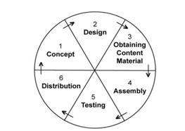
Figure 4. Multimedia Development Life Cycle.

2.3. Insertion sorting

Although the Insertion Sorting is not like the bubble sorting and the selection sorting, it is a little complex. The insertion sorting also has an optimization algorithm called split and half insertion.

The step of the algorithm is that treat the first element of sequence which will be sorted as an ordered sequence, and treat the second element through the last element as an unordered sequence. Scan the unordered sequence from the first to the last, inserting every element which is scanned into its proper place in the ordered sequence. If the element which would be inserted is equal to one of the elements in the ordered sequence, the element which will be inserted should be put behind the equal element.

Consider a list of numbers: 2, 5, 8, 3, 6, 9, 1, 4, 7

First, just think of 2 as ordered, and the left numbers are unordered. Then choose the first element of unordered sequence 5. Compare it with 2. It is greater than 2. So put it behind 2. And then is 8, 8 is greater than 2 and 5, so put it behind them.2,5,8 is ordered now. Then when it comes to 3, 3 is only greater than 2 while it is less than 5 and 8, so put it behind 2. It is 2,3,5,8 now. Next, choose 6, 6 is only smaller than 8, so put it behind 8, the order now is 2,3,5,6,8. The steps are like this, first, choose the unordered element, if it is smaller than the ordered elements, then it needs to be put behind it, otherwise put it in front of it. So the final order is 1,2,3,4,5,6,7,8,9.

The Insertion Sort Algorithm can be applied in a typical way using the Bidirectional Conditional Insertion Sort algorithm. This algorithm shortens the operations caused by insertion processes with new skills. It could be find that there are two aligned parts on the left and right of the array, and the misaligned part is between the two aligned parts.[5]. If the algorithm sorts increasingly,the left part will put the smallest element while the right part order the greatest element. Inversely, the smaller one will be located on the right and the larger one will be on the left.

The biggest difference between BCIS and the classical algorithm is that the insertion of items into two parts could help save cost on the memory read and the write operations as the length of the Insertion sort is distributed into two sorted parts in Bidirectional Conditional Insertion Sort. It could also put at least one object in the right position during a trip.

The complexity of this algorithm depends on the complexity of insertion functions, to be clear, on the number of elements inserted in each sorting process. To simplify this analysis, the main part of the algorithm should be emphasized.Hypothesize that there are k elements in total to be inserted into both sides, there are k/2 elements on each side. The principle of the insertion function works very like standard insertion sort. So the left side adds the right side is the outcome of time complexity. Each function is T(k/2), so it could be expressed as the figure 5

The complexity of insertion functions and the value k could determine the complexity of algorithm.

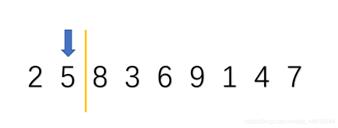
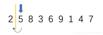
Figure 5. The steps of the insertion sort.

2.4. Hill sort

Hill sort is also known as the reduction increment method. The basic idea of Hill Sort is that Select an integer and divide all records in the file to be sorted into multiple groups. All the records with a distance of 1 are grouped in the same group, and the records in each group are directly inserted into the sort. Then take and repeat the above grouping and sorting work. When the gap is equal to 1, all the records are sorted within the unified group. That is to say, Hill Sort makes data into groups, placing groups in an insertion sort. After each group is arranged in order, the whole data becomes ordered. The gap is the ratio of elements to sorting time.

Take 9,1,2,5,7,4,8,6,3,5 as an example

There are 10 elements in total. Do the first sorting

The gap is equal to 10/2=5. So 9 and 4, 1 and 8, 2 and 6, 5 and 3, 7 and 5 are groups and then sort them respectively. Put the smaller one in front of the larger one. And the order is that 4,1,2,3,5,9,8,6,5,7. Then do the second sort, the gap is equal to 10/22=2, so 4 and 2, 1 and 3, 2 and 5, 3 and 9, 5 and 8, 9 and 6, 8 and 5, 6 and 7. The next order is that 2,1,4,3,5,6,5,7,8,9. Then the gap is equal to 10/23=1. So the final order is that 1,2,3,4,5,5,6,7,8,9. This is principle of the hill sort.

Hill sort is an optimization of direct insertion sort. The feature of the direct insertion sort is that the more ordered data, the faster it is. If the gap is greater than 1, it is called pre-sorted, the purpose is to make the array closer to order. When the gap is equal to 1, the array is closed to order, so it will be faster. In this way, the overall effect can be optimized. Then compare the performance test after implementation.

To be honest, the time complexity of hill sort is not easy to calculate, as there are a lot of ways to value the gap, which is not easy to calculate. The time complexity of Hill sort is not fixed. Some scholars calculate it through a large number of experimental statistics, the result is O(n1.25)-O(1.6*n1.25). The space complexity of it is O(1).

Those elements are not adjacent and their position of them are switched. So the algorithm is not stable.

The code of hill sort is that(see figure 6):

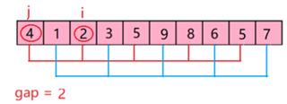
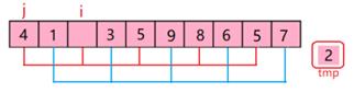
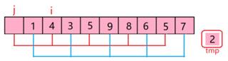
Figure 6. The principle of hill sort.

2.5. Merge sort

The merge operation is used to create an efficient sorting algorithm called Merge sort, which is a common use for Divide and Conquer. Merge the sorted subsequence to get a entire ordered sequence; first, order each subsequence first, second, order the subsequence segments.

There are two basic ideas about the merge sort. The first one is the splitting, and this is the procedure of dividing the original array into two subarrays. The other one is the partition, which merges those two ordered arrays into a larger ordered array.

The linear table that needs to be sorted is broken down into multiple sub-tables until there is only one element in each sub-table. In this case, it can be considered that a sub-table contains only one element in an ordered table.

Merge the child table in pairs. Each time the child table is merged, a new and longer-ordered table is produced. Do this step repeatedly until there is one child table left, which is the sorted linear table.

Take 8,4,5,7,1,3,6,2 as an example.

First, divide this data into two parts 8,4,5,7 and 1,3,6,2. Also, divide 8,4,5,7 into 8 and 4; 5 and 7; divide 1,3,6,2 into 1 and 3; 6 and 2. Compare them respectively, the first part is 4,5,7,8 and the second part is 1,2,3,6.

Think 4 as i and think 1 as j, 1 is smaller than 4 so put it in front of 4 then think 2 is j, 2 is also smaller than 4, put it in front of 4 and behind 1. Consider 3 as j, 3 is smaller than 4. So put it behind 2. Lastly think about 6, 6 is greater than 4 and 5, so put it behind 5.

The merge sort algorithm and selection sorting and merge sorting's performance are shown in Figures 7 and 8.

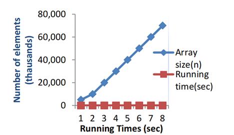
Figure 7. Running times of merge sort algorithm.

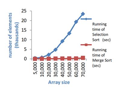
Figure 8. Performance of selection sort and merge sort algorithms.

When the array size is around 10,000, the time required is 0.712s, but when it increases to 20,000, it becomes clear. Meanwhile the time needed becomes 2.140s[6]. In addition, it is also obvious that when the array size ranges from 30,000 to 40,000 elements. Running time of 4000 elements is about four times more than 3000 elements. From those two figures, it can be found that the merging sort algorithm shows better on both smaller and greater array sizes compared with the selection sort algorithm in all of those processes. Just as the findings of Rabiu et al[7] and Aliyu and Zirra [8]. The input size of the array counts on the performance of the algorithms. The time complexity which is O(log (n)) just as the merge sort performs better than those time complexity is O(n2) just like the selection sorting. This opinion corresponds with the findings of Thomas et al[9]; Rabiu et al[10].

The table1 shows the comparison of different algorithms.

Table 1. Comparison of different algorithms.

3. Conclusion

In conclusion, the sorting algorithms including bubble sort, insertion sort, selection sort, hill sort, and merge sort play an important role in the field of scientific research and even daily life. The time complexity could be used to calculate the running time of a program, compare efficiency of algorithms, and help researchers decide which one would be done first and arrange a time for the best. Also, the time complexity could optimize the design of the algorithm by recognizing which algorithm has the lowest efficiency and which one has the highest efficiency and then revising them, improving the characteristics of the algorithms. For example, when it comes to problems that need to be solved quickly and the data scale is large, algorithms with lower time complexity could be the best option. The algorithm also has space complexity which could measure how much storage space an algorithm temporarily takes up during its run. It is primarily concerned with how much additional storage space the algorithm requires in addition to input data when it is executed, especially those that are dynamically applied for when it is running. The rules for the space complexity are similar to the rules for the time complexity, using the big O asymptotic notation, which does not simply count how many bytes of space the program occupies, but the number of variables, as this is the more critical for analyzing the performance of the algorithm.

There are many ways and directions for the algorithms to be applied in the future. The most popular one is using sorting algorithms to optimize the resource such as the search algorithm, by optimizing the sorting process of the algorithm, then improving the efficiency of the algorithms and programs. Also, algorithms tend to be used to evaluate the grades of employees. Choosing an aspect as a standard. Arranging them from the best to the lowest. It can help companies organize staff better.

References

[1]. Bentley, J. L., & Sedgewick, R. (1997, January). Fast algorithms for sorting and searching strings. In Proceedings of the eighth annual ACM-SIAM symposium on Discrete algorithms (pp. 360-369).
[2]. Jie, L., Zheng, B., & Flynn, M. P. (2019, February). 20.3 A 50MHz-bandwidth 70.4 dB-SNDR calibration-free time-interleaved 4 th-order noise-sha** SAR ADC. In 2019 IEEE International Solid-State Circuits Conference-(ISSCC) (pp. 332-334). IEEE. doi:10.1109/ISSCC.2019.8662313.
[3]. Fan, H., Liu, Y., & Feng, Q. (2020). A reliable bubble sorting calibration method for SAR ADC. AEU-International Journal of Electronics and Communications, 122, 153227.
[4]. Sutopo, H. (2011). Selection sorting algorithm visualization using flash. The International Journal of Multimedia & Its Applications (IJMA), 3(1), 22-35.
[5]. Mohammed, A. S., Amrahov, Ş. E., & Çelebi, F. V. (2017). Bidirectional Conditional Insertion Sort algorithm; An efficient progress on the classical insertion sort. Future Generation Computer Systems, 71, 102-112.
[6]. Rabiu, A. M., Garba, E. J., Baha, B. Y., & Mukhtar, M. I. (2021). Comparative analysis between selection sort and merge sort algorithms. Nigerian Journal of Basic and Applied Sciences, 29(1), 43-48.
[7]. Rabiu, A.M., Garba, E.G., Baha, B.Y. & Mukhtar, M.I. (2020). Optimizing frameworks for building more efficient concurrent application in Java.Islamic University Multidisciplinary Journal (IUMJ), 7(2):348-355.
[8]. Aliyu, A. M. & Zirra, P. B. (2013). A comparative analysis of sorting algorithms on integerand character arrays. The International Journal of Engineering and Science, .2(7): 25-30.
[9]. Thomas, H. C., Charles, E. L., Ronald, L. R. & Clifford, S. (2004). Introduction to Algorithms (4th Ed.).NY: AddisonWesley Professional, 50-51.
[10]. Rabiu, A.M., Garko, A.B., &Abdullahi, A.M. (2018).Effects of multi-core processors on linearand binary sorting algorithms.Dutse Journal of Pure and Applied Sciences, 2(4):130-140
Cite this article
Liu,P. (2024). An in-depth study of sorting algorithms. Applied and Computational Engineering,92,187-195.
Data availability
The datasets used and/or analyzed during the current study will be available from the authors upon reasonable request.
Disclaimer/Publisher's Note
The statements, opinions and data contained in all publications are solely those of the individual author(s) and contributor(s) and not of EWA Publishing and/or the editor(s). EWA Publishing and/or the editor(s) disclaim responsibility for any injury to people or property resulting from any ideas, methods, instructions or products referred to in the content.
About volume
Volume title: Proceedings of the 6th International Conference on Computing and Data Science
© 2024 by the author(s). Licensee EWA Publishing, Oxford, UK. This article is an open access article distributed under the terms and
conditions of the Creative Commons Attribution (CC BY) license. Authors who
publish this series agree to the following terms:
1. Authors retain copyright and grant the series right of first publication with the work simultaneously licensed under a Creative Commons
Attribution License that allows others to share the work with an acknowledgment of the work's authorship and initial publication in this
series.
2. Authors are able to enter into separate, additional contractual arrangements for the non-exclusive distribution of the series's published
version of the work (e.g., post it to an institutional repository or publish it in a book), with an acknowledgment of its initial
publication in this series.
3. Authors are permitted and encouraged to post their work online (e.g., in institutional repositories or on their website) prior to and
during the submission process, as it can lead to productive exchanges, as well as earlier and greater citation of published work (See
Open access policy for details).