


1. Introduction
Heart disease is a kind of disease with high morbidity and high mortality, which is a major killer threatening the life and health of contemporary human beings, especially the middle-aged and elderly people over 50 years old [1]. ECG signal, Electrocardiogram signal, is an important data for monitoring human heart condition, prevention and treatment of heart disease. Studying the relationship between the characteristics of ECG signal and heart health status can provide an efficient and accurate statistical tool for preventing heart disease earlier and more effectively, which has wide practical and social significance. ECG signal classification is mainly divided into three steps: data preprocessing, feature extraction, and classifier selection and training [2]. In recent years, with the development of artificial intelligence and machine learning, there have been many algorithms based on support vector machines, random forest, etc., which can be used for this classification task. Yeh et al. [3] proposed a method to classify ECG data of arrhythmia using cluster analysis. They detected QBS wave groups and extracted features. This method could effectively classify normal heart beats and four abnormal heart beats, achieving an average accuracy of 94.30%. Li et al. [4] used wavelet transform to decompose ECG signals, then calculated the entropy of different components as representative features into the random forest for classification, and improved the generalization ability of the classifier among different patients by dividing the training set and the test set respectively for each patient. Varatharajan et al. [5] used a linear discriminant dimensionality reduction (LDA) method to filter the data features, and classified the ECG signal data by a support vector machine (SVM) with enhanced kernel. This method can achieve better classification results and can adapt to the environment of big data and cloud computing. Liu Shu et al. [6] proposed a method to extract ECG signal features by using bispectral matrix and graph Fourier transform. The bispectral matrix was transformed into the feature range by using graph Fourier transform, and then the graph features were extracted directly, overcoming the computational defects of traditional bispectral matrix method. At the same time, with the improvement of computing power, the methods of classifying ECG signals using deep learning and neural network are also emerging in endlessly. Kiranyaz et al. [7] applied one-dimensional convolutional neural networks (CNNS) to feature extraction and classification tasks to develop a special CNNS for each patient, which can be quickly and accurately applied to long-term ECG signal streams, and thus can be applied to real-time classification of patients' ECG data. However, there are some obvious problems with the above approach. First of all, ECG signal is a kind of nonlinear, non-stationary weak signal, the frequency is concentrated between 0.25-35Hz, and the ECG signal collected in the medical field is often easy to mix with a lot of noise, so that the signal to noise ratio of the signal is greatly reduced, these characteristics will increase the difficulty of its classification, and have an adverse impact on the final classification result; In addition, most of the deep learning algorithms based on neural networks are not strong in interpretation, and can not provide an effective basis for doctors' diagnosis. Therefore, this paper firstly uses discrete wavelet transform to screen signals from two dimensions of frequency and time to improve signal to noise ratio. Then XGBoost model is used for classification, and according to the information gain of each feature in the training process as the importance index of the feature, the focus of attention to distinguish the abnormal types of heart rate is obtained, the interpretability of the model is improved, and the reference is provided for manually distinguishing the abnormal types.
2. Method
2.1. Discrete Wavelet transform
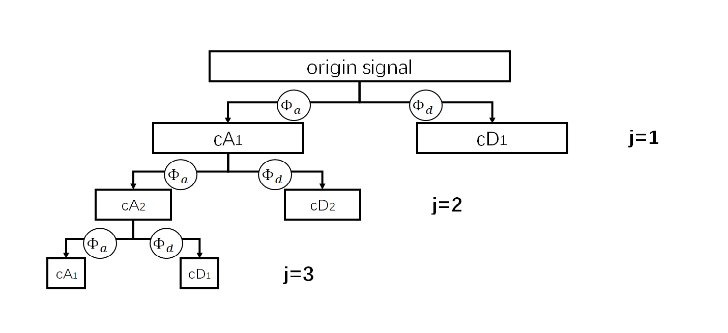
ECG signal is easy to be mixed with a lot of noise during acquisition, such as baseline drift, myoelectric interference, power frequency noise, etc. [8]. Baseline drift is the main noise of ECG signal, mainly caused by the patient's breathing, electrode patch sliding and other factors, the frequency is very low, generally less than 1Hz; Myoelectric interference is the noise generated by human muscle trembling, and the frequency is generally between 10-1000Hz; Power frequency noise refers to the noise caused by medical devices and the surrounding environment, and its frequency is 50-60Hz. If the above noise is not removed, it may mask the true waveform of the ECG signal, resulting in signal distortion and degraded model classification. Wavelet Transformation is a mathematical tool widely used in the field of signal analysis. Its principle is to convolve wavelet functions of different parameters with the original signal to extract the information of the signal at different time and frequency scales [9]. Compared with the trigonometric function, the wavelet function does not have periodicity in the whole real number field, but has different amplitudes in different locations, so the translation and extension of the wave function and then convolution with the original signal can get the information of the original signal in different time domain. Its mathematical definition is as follows: \[C_{a,b}(f)=\frac{1}{\sqrt{|a|}}\int_{-\infty}^{\infty}f(t)\Phi (\frac{t-b}{a}) \mathrm{d}t\] Where \(\Phi(t)\) is the wavelet function and \(f\) is the original signal. Discrete Wavelet Transformation (DWT) decompose the signal into high frequency detail and low frequency overview by selecting wavelet functions with different parameters. Each subsequent layer is decomposed from the previous layer. So that the signal can be analyzed at different frequencies and time scales, and its mathematical definition is \[cA_j=\{\frac{1}{\sqrt{2^j}}\sum_{t=0}^{T}cA_{j-1}(t)\Phi_a(\frac{t-k\cdot2^j}{2^j})\}_{1\leq k \leq [T/2^j]} ,j=1,2,...\] \[cD_j=\{\frac{1}{\sqrt{2^j}}\sum_{t=0}^{T}cA_{j-1}(t)\Phi_d(\frac{t-k\cdot2^j}{2^j})\}_{1\leq k \leq [T/2^j]} ,j=1,2,...\] Where \(cA_j\) and \(cD_j\) the general part and the detail part of the \(j\) th layer respectively,Denote that \(cA_0=f\) , \(\Phi_a\) and \(\Phi_d\) are the corresponding wavelet functions of the two parts, \(\{f(t)\}_{1\leq t\leq T}\) is the discretization of the original signal, the specific decomposition process is shown in Figure 1.
Discrete wavelet transform denoising , that is, to use of discrete wavelet transform to decompose the original data, after which denoise each part of the decomposition and then reassemble the original signal process. That's to say , for the part \(cD_1,cD_2,...,cD_l,cA_l\) obtained by the \(L\) -layer decomposition of signal \(f\) ,let
S_i(x)-\delta \cdot max{S_i} x\gt \delta \cdot max\{S_i\}
\end{aligned} . \end{equation}
where \(\delta\) is artificially set threshold. Then the denoising step will be finished after reassembe all those denoised parts.
2.2. XGBoost
XGBoost(full name eXtreme Gradient Boosting) is an efficient implementation of gradient Boosting tree (GBDT), which greatly improves the running efficiency of the algorithm by gradient approximation method, and has unique advantages in handling large-scale data. At the same time, the addition of L1 and L2 regular terms can effectively avoid overfitting problems and improve the generalization ability of the model.
XGBoost is designed to train an additive model for regression tree integration, which can be expressed as:
\[\hat{y}=f(x)=\sum_{k=1}^{M} f_k(x)\]
In the above formula, \(f_k(x),k=1,2,...,M\) is M different regression trees, XGBoostuses greedy algorithm when training these trees, that is, adding and training one tree at each step, fixing all the previous trees. At step t, let the first t-1 trees be trained and fixed, and if the loss function for a single sample is \(l(y,\hat{y})\) , then XGBoost adopts the objective function of
\begin{align*}
Obj^{(t)}&=\sum_{i=1}^{n} l\left(y_i,f(x_i)\right)+\Omega(f_t)
&=\sum_{i=1}^{n} l\left(y_i,\hat{y}_i^{(t-1)}+f_t(x_i)\right)+\Omega(f_t)
\end{align*}
where \(\hat{y}_i^{(k-1)}=\sum_{k=1}^{t-1} f_k(x_i)\) is the predicted result of the former t-1 tree, and \(\Omega(f_t)\) is the penalty term for model complexity, defined as:
\[\Omega(f)=\gamma T+\frac{1}{2}\lambda \sum_{j=1}^T w_j^2\]
where \(T\) stands for the number of leaf nodes of tree \(f\) , \(w_j,j=1,2,...,T\) stands for the return values of them.
In order to reduce the amount of computation of gradient descent, the algorithm adopts second-order Taylor expansion to approximate the objective function as a quadratic function:
\[\mathcal{L}^{(t)} \approx \sum_{i=1}^n [l(y_i,\hat{y}_i^{(t-1)})+\frac{
tial}{
tial \hat{y}} l(y_i,\hat{y}_i^{(t-1)})f_t(x_i)+\frac{1}{2} \frac{
tial^2}{
tial \hat{y}^2} l(y_i,\hat{y}_i^{(t-1)})f_t^2(x_i)]+\Omega(f_t)\]
Note that the first term in the sum is a constant, denote
\[g_i=\frac{
tial}{
tial \hat{y}} l(y_i,\hat{y}_i^{(t-1)})\]
\[h_i=\frac{
tial^2}{
tial \hat{y}^2} l(y_i,\hat{y}_i^{(t-1)})\]
Let \(I_j\) be the subscript set of the sample belonging to the \(j\) th leaf node, then the above equation can be further simplified to
\&= \sum_{i=1}^n [ g_i f_t(x_i)+\frac{1}{2}h_i f_t^2(x_i)]+\gamma T_t+\frac{1}{2}\lambda \sum_{j=1}^{T_t} w_{tj}^2+const
\&= \sum_{j=1}^{T_t}[(\sum_{i \in I_j}g_i)w_{tj}+\frac{1}{2}(\sum_{i \in I_j}h_i+\lambda)w_{tj}^2]+\gamma T_t+const \end{align}
Let \(G_j=\sum_{i \in I_j}g_i\) , \(H_j=\sum_{i \in I_j}h_i\) when the t th tree has been divided and determined, in order to minimize the objective function, the value of each leaf node should be \(w_{tj}=-\frac{G_j}{H_j+\lambda},j=1,2,...,T_t\) , when the objective function value is \(-\frac{1}{2}\sum_{j=1}^{T_t}\frac{G_j^2}{H_j+\lambda}+\gamma T_t\) . When determining the structure of the tree, at each step, determine whether to split according to the loss comparison before and after the node splits, such as deciding whether to split node A into B and C, calculate the gain: \[\mathcal{L}_{split}=\frac{1}{2}[\frac{(\sum_{i \in I_B} g_i)^2}{\sum_{i \in I_B} h_i+\lambda}+\frac{(\sum_{i \in I_C} g_i)^2}{\sum_{i \in I_C} h_i+\lambda}-\frac{(\sum_{i \in I_A} g_i)^2}{\sum_{i \in I_A} h_i+\lambda}]-\gamma\] When the gain is positive, the node is split; Otherwise it does not.
3. Experiment
3.1. Experimental Environment
All experiments in this paper are implemented using Python3.9.18 programming, Jupyter Notebook as the platform, and AMD Ryzen 7 5800H with Radeon Graphic CPU. Model training was carried out on a computer with NVIDIA Geforce RTX 3060 GPU with 16GB running memory. Detailed configuration parameters are shown in Table 1. The main part of the experiment, namely noise reduction by discrete wavelet transform and XGBoost classification, is implemented based on pywt library and scikt-learn library of Python.
Table 1: Details of experimental environment
| Element | Version |
|---|---|
| CPU | AMD Ryzen 7 5800H with Radeon Graphic |
| GPU | NVIDIA Geforce RTX 3060 |
| Operating system | Windows11 64bit |
| Memory | 16G(3200MHz) |
| Programming language | Python3.9.18 |
| Platform | Jupyter Notebook |
3.2. Data Preprocessing
An ECG signal, or electrocardiogram signal, is a time series obtained by collecting the electrical signals generated during periodic fluctuations in the human heart. The signal generated by a cycle of cardiac activity is called a "beat". The general beat data consists of P wave, QRS complex wave, T wave and other specific waveforms, and its schematic waveform is shown in Figure 2 :
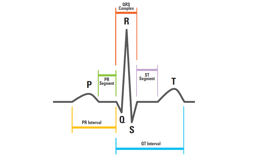
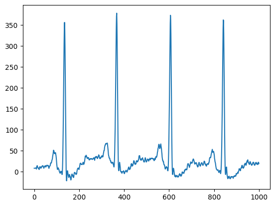
The P wave is the first wave of the beat cycle, which is generated by atrial excitation and reflects the potential changes in the process of atrial muscle depolarization; QRS complex wave is the highest amplitude band in electrocardiogram, consisting of Q wave, R wave and S wave, which reflect the potential changes in the process of ventricular excitation. R wave is generally short and has the highest amplitude, and can be used to locate the position of the beat in the entire electrocardiogram. T wave is the wave at the end of the beat, the amplitude should not be less than 1/10 of the concentric beat R wave, reflecting the potential change of ventricular repolarization. The data used in this paper came from MIT-BIH database, which was provided by the Massachusetts Institute of Technology and recorded the heart rate changes of 48 patients in Beth Israel Hospital during 1975-1979. It is the most widely used ECG database in the world [10]. Each piece of data is a patient's ECG data over a long period of time, which contains multiple beats (see Figure 2 for example). The R-wave position of each beat and the type of the beat are marked in the data. In order to save training costs, five of the most frequently occurring heart beats were selected in this experiment. Their marks and meanings are shown in Table 2.
Table 2: Labels and their meaning
| Labels | Meaning |
|---|---|
| N | Normal beat |
| L | Left bundle branch block beat |
| R | Right bundle branch block beat |
| / | Paced beat |
| A | Aberrated atrial premature beat |
| V | Premature ventricular contraction |
| Q | Unclassifiable beat |
| f | Fusion of paced and normal beat |
In order to keep the position of each waveform in the beat relatively fixed, this experiment selected each R wave 100 unit time forward and 150 unit time backward as one beat. A total of 82,837 heart beat samples were obtained, among which the largest category was 69.3% normal (N) heart beat, and the frequencies of other abnormal heart beats were shown in Figure 4.
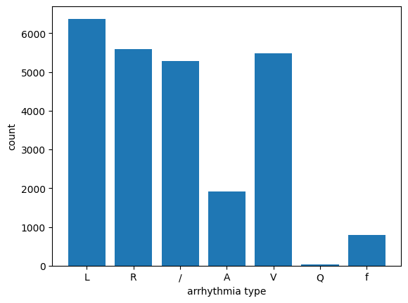
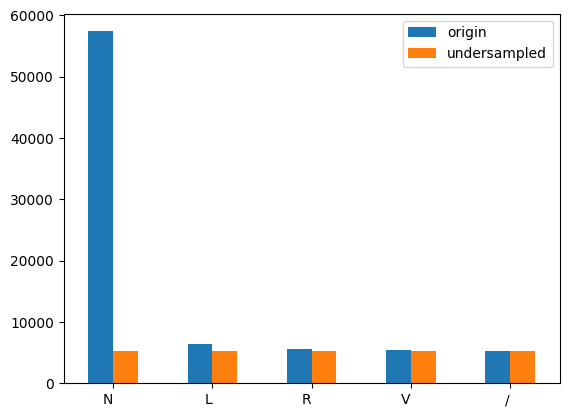
Five of the most common types of beats, including normal beats, were selected as the dataset, namely normal beats (N), left bundle branch block (L), right bundle branch block (R), ventricular premature beat (V) and pacemaker heartbeat (/). In order to solve the problem of sample imbalance with large proportion of normal beats, undersampling method was adopted, and the number of samples of the class with the smallest number of samples (pacing heartbeat) was taken as the benchmark, and the same number of samples of other types were taken as the new data set. The comparison of effects before and after undersampling was shown in Figure ref{fig5}.
3.3. Comparative experiment
3.3.1. Discrete wavelet transform
In order to determine the optimal threshold of discrete wavelet transform, four indexes of accuracy, precision, recall and F1 score were selected in the experiment. The effect of training XGBoost classifier with noise reduction data under each threshold was attempted by using the method of 50% cross verification. The experimental results are shown in Table 3:
Table 3: result of thresholds
| threshold | accuracy | precision | recall rate | F1 score |
|---|---|---|---|---|
| 0.0 | 0.9882 | 0.9882 | 0.9882 | 0.9882 |
| 0.01 | 0.9885 | 0.9885 | 0.9885 | 0.9885 |
| 0.02 | 0.9881 | 0.9881 | 0.9881 | 0.9881 |
| 0.03 | 0.9882 | 0.9883 | 0.9882 | 0.9882 |
| 0.04 | 0.9882 | 0.9882 | 0.9882 | 0.9882 |
| 0.08 | 0.9889 | 0.9889 | 0.9889 | 0.9889 |
| 0.12 | 0.9884 | 0.9884 | 0.9884 | 0.9884 |
| 0.16 | 0.9874 | 0.9875 | 0.9874 | 0.9874 |
| 0.18 | 0.9874 | 0.9874 | 0.9874 | 0.9874 |
| 0.22 | 0.9874 | 0.9875 | 0.9874 | 0.9874 |
| 0.26 | 0.9866 | 0.9866 | 0.9866 | 0.9866 |
| 0.3 | 0.9866 | 0.9866 | 0.9866 | 0.9866 |
It can be seen that when the appropriate threshold is selected, the noise reduction by discrete wavelet transform has a certain improvement effect on the classification effect, and the classification effect is the best when \(\delta=0.08\) .Therefore, the data set under the noise reduction of this threshold will be fixed as the experimental data set in the subsequent experiments.
3.3.2. XGBoost classification
The parameter Settings of the XGBoost learner used in the experiment are shown in Table 4.
Table 4: Parameter settings of XGBoost
| symbols | value | meaning |
|---|---|---|
| \(M\) | 100 | number of regression trees |
| \(\lambda\) | 3 | penalty coefficients for values of leaf nodes |
| \(\gamma\) | 0 | penalty coefficients for number of leaf nodes |
| \(\eta\) | 0.1 | learning rate |
| \(D_{max}\) | 6 | the maximum depth of trees |
| \(p\) | 5 | class number |
| \(l\) | Cross Entropy Loss | loss function of a single sample |
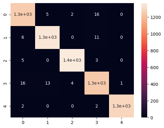
The data was randomly divided into 25% test set and 75% training set, and the accuracy of the final prediction result was 98.7%, and the confusion matrix was shown in Figure 6. It can be seen that the classifier has achieved a very good classification effect, most of the samples of each type are classified correctly, and the distribution of classification error samples is relatively high. Uniform, basically no large-scale mismarking.
3.4. Feature Importance
Although machine learning methods have achieved good results in many fields, they are often less explanatory than traditional statistical models. In order to make up for this shortcoming, this paper discusses the importance of each feature in the classifier training process, and draws relevant conclusions based on it. In the process of training XGBoost, the importance of features is mainly reflected in the information gain of the classification task, so it is defined that the importance of a feature is proportional to the decline value of the loss function every time the node is split according to the feature, that is, the sum of the split gain \(\mathcal{L}_{split}\) . The importance of the 250 features obtained from this is shown in Figure 7.
It is noted that the R-wave position is fixed at the 101st feature when splitting the heart beat, so it can be seen from the figure above that the important features are concentrated at the rear end of the QRS-wave group and the T-wave position at the end. This indicates that the difference between these two waveforms should be paid attention to when manually distinguishing the abnormal heartbeat waveforms.
3.4.1. Compared with other models
To compare the results of XGBoost, several other common machine learning classifiers were tried: RandomForest, support vector machine (SVM), one-dimensional convolutional neural network (1dCNN). Their main parameter Settings are shown in Table 5.
Table 5: Main parameters of other learners
| Random Forest | Support vector machine | convolutional neural network |
|---|---|---|
| \makecell{ \(n\_estimators=120\) \(max\_features=15\) \__escape_dollar__criterion=gini \(}\lt /td\gt \lt td style="text-align: right"\gt \makecell{\) kernel=rbf \(\lt br\gt \) C=1.0 \(}\lt /td\gt \lt td style="text-align: center"\gt \makecell{\) lr=0.0002 \(\lt br\gt \) num\_epoch=10$} |
The architecture of one-dimensional convolutional neural network (1dCNN) is shown in Table 6 [11].
Table 6: Architecture of 1dCNN
| sequence | parameters | kernel size | activation function | dimension of output |
|---|---|---|---|---|
| 1 | Conv1d(1,32) | 5 | ReLU | 246*32 |
| 2 | AvgPool1d | 2 | - | 123*32 |
| 3 | Conv1d(32,32) | 4 | ReLU | 120*32 |
| 4 | AvgPool1d | 2 | - | 60*32 |
| 5 | Conv1d(32,32) | 5 | ReLU | 56*32 |
| 6 | AvgPool1d | 2 | - | 28*32 |
| 7 | Conv1d(32,32) | 5 | ReLU | 24*32 |
| 8 | AvgPool1d | 2 | - | 12*32 |
| 9 | Conv1d(32,32) | 3 | ReLU | 10*32 |
| 10 | AvgPool1d | 2 | - | 5*32 |
| 11 | Flatten | - | - | 160 |
| 12 | Linear(160,32) | - | ReLU | 32 |
| 13 | Linear(32,5) | - | ReLU | 5 |
| 14 | Softmax | - | - | 5 |
The data after noise reduction with the optimal threshold of 0.08 selected above is selected, and the training set and data set are divided according to 75% and 25%, and the above classifier is trained. The performance on the test set is shown in Table 7.
Table 7: results of learners
| learner | accuracy | precision | recall rate | F1 score |
|---|---|---|---|---|
| XGBoost | 0.9870 | 0.9870 | 0.9870 | 0.9870 |
| Random Forest | 0.9864 | 0.9864 | 0.9864 | 0.9864 |
| SVM | 0.9815 | 0.9815 | 0.9815 | 0.9815 |
| 1dCNN | 0.9710 | 0.9711 | 0.9710 | 0.9710 |
It can be seen that XGBoost has significant advantages in solving ECG signal classification problems compared with other machine learning models, and its algorithm runs fast, has little randomness, is strong in interpretation, and has the best synthesis.
4. Conclusion
In this paper, we use MIT-BIH arrhythmia database as experimental data set, combined with DWT noise reduction and Xgboost to study ECG signal classification. In the data preprocessing stage, we firstly locate the heart beat position through R wave, divide the data set into a single heart beat according to one heart beat every 250 unit time, then select the five heart beats with the highest frequency, and compose the sample balanced experimental data after undersampling. In the noise reduction stage of discrete wavelet transform, we compared the noise reduction effect of discrete wavelet transform under different thresholds through the five-fold cross-validation and five indicators, and comprehensively selected 0.08 as the best noise reduction threshold. After obtaining the data set of the previous step, we divided the data set into the training set and the test set according to the ratio of 3:1 to train the XGBoost classifier, and finally got 98.7% of the correct rate on the test set and the confusion matrix with more balanced errors. Finally, according to the information gain in the training process of Xgboost, we carry out the feature importance analysis of the experiment, and get the conclusion that we should pay attention to the back end of QRS wave and T wave to distinguish heartbeat anomaly. Although the method in this paper has achieved good classification effect, there are still some problems. For example, the classification model in this paper is a single model, so it may not be robust enough in some special cases, and it is difficult to generalize good results. Future work may consider training and classification in the environment of multiple classifiers such as model integration, in order to pursue better generalization and robustness.
References
[1]. Guo Jianning and Li Wei. “Analysis of common cardiovascular and cerebrovascular diseases in elderly emergency patients”. In: Electronic Journal of Integrated Traditional and Western Medicine Cardiovascular Diseases 3.35 (2015), p. 2.
[2]. Liang Yisong. “Arrhythmia classification and signal time scale based on Deep learning”. MA thesis. Shandong University, 2024.
[3]. Yun-Chi Yeh, Che Chiou, and Lin Hong- Jhih. “Analyzing ECG for cardiac arrhythmia using cluster analysis”. In: Expert Systems with Applications: An International Journal 39 (Jan. 2012), pp. 1000–1010. DOI: 10.1016/j.eswa.2011.07.101.
[4]. Taiyong Li and Min Zhou. “ECG Classification Using Wavelet Packet Entropy and Random Forests”. In: Entropy 18 (Aug. 2016), p. 285. DOI: 10.3390/e18080285.
[5]. Ramachandran Varatharajan, Gunasekaran Manogaran, and Priyan M K. “A big data classification approach using LDA with an enhanced SVM method for ECG signals in cloud computing”. In: Multimedia Tools and Applications 77 (Nov. 2017). DOI: 10.1007/s11042-017-5318-1.
[6]. Liu Shu et al. “Ecg signal classification based on bispectral and spectral features”. In: Electronic Science and Technology (2021).
[7]. Serkan Kiranyaz, Turker Ince, and Moncef Gabbouj. “Real-Time Patient-Specific ECG Classification by 1-D Convolutional Neural Networks”. In: IEEE Transactions on Biomedical Engineering 63.3 (2016), pp. 664–675. DOI: 10.1109/TBME.2015.2468589.
[8]. Chen Siyu. “Research on ECG signal denoising, Wave group detection and arrhythmia recognition algorithm”. MA thesis. Place of publication unknown]: Nanjing University of Finance and Economics, 2024.
[9]. Zhu Jinling. “Application of wavelet threshold denoising technology in ECG signal processing”. In: China High-Tech (2022), pp. 88–89. ISSN: 2096-4137. DOI: 10.13535/j.cnki.10- 1507/n.2022.04.36.
[10]. Song Xiguo and Deng Qinkai. “Understanding and application of MIT-BIH arrhythmia database”. In: Chinese Journal of Medical Physics 21.4 (2004), p. 3.
[11]. Cheng Xiangqian. “ECG signal classification based on fusion of CNN and SVR evidence theory”. MA thesis. Shandong University of Science and Technology, 2021.
Cite this article
Yu,X. (2024). ECG signal classification based on DWT denoising and XGBoost. Applied and Computational Engineering,95,57-67.
Data availability
The datasets used and/or analyzed during the current study will be available from the authors upon reasonable request.
Disclaimer/Publisher's Note
The statements, opinions and data contained in all publications are solely those of the individual author(s) and contributor(s) and not of EWA Publishing and/or the editor(s). EWA Publishing and/or the editor(s) disclaim responsibility for any injury to people or property resulting from any ideas, methods, instructions or products referred to in the content.
About volume
Volume title: Proceedings of the 6th International Conference on Computing and Data Science
© 2024 by the author(s). Licensee EWA Publishing, Oxford, UK. This article is an open access article distributed under the terms and
conditions of the Creative Commons Attribution (CC BY) license. Authors who
publish this series agree to the following terms:
1. Authors retain copyright and grant the series right of first publication with the work simultaneously licensed under a Creative Commons
Attribution License that allows others to share the work with an acknowledgment of the work's authorship and initial publication in this
series.
2. Authors are able to enter into separate, additional contractual arrangements for the non-exclusive distribution of the series's published
version of the work (e.g., post it to an institutional repository or publish it in a book), with an acknowledgment of its initial
publication in this series.
3. Authors are permitted and encouraged to post their work online (e.g., in institutional repositories or on their website) prior to and
during the submission process, as it can lead to productive exchanges, as well as earlier and greater citation of published work (See
Open access policy for details).
References
[1]. Guo Jianning and Li Wei. “Analysis of common cardiovascular and cerebrovascular diseases in elderly emergency patients”. In: Electronic Journal of Integrated Traditional and Western Medicine Cardiovascular Diseases 3.35 (2015), p. 2.
[2]. Liang Yisong. “Arrhythmia classification and signal time scale based on Deep learning”. MA thesis. Shandong University, 2024.
[3]. Yun-Chi Yeh, Che Chiou, and Lin Hong- Jhih. “Analyzing ECG for cardiac arrhythmia using cluster analysis”. In: Expert Systems with Applications: An International Journal 39 (Jan. 2012), pp. 1000–1010. DOI: 10.1016/j.eswa.2011.07.101.
[4]. Taiyong Li and Min Zhou. “ECG Classification Using Wavelet Packet Entropy and Random Forests”. In: Entropy 18 (Aug. 2016), p. 285. DOI: 10.3390/e18080285.
[5]. Ramachandran Varatharajan, Gunasekaran Manogaran, and Priyan M K. “A big data classification approach using LDA with an enhanced SVM method for ECG signals in cloud computing”. In: Multimedia Tools and Applications 77 (Nov. 2017). DOI: 10.1007/s11042-017-5318-1.
[6]. Liu Shu et al. “Ecg signal classification based on bispectral and spectral features”. In: Electronic Science and Technology (2021).
[7]. Serkan Kiranyaz, Turker Ince, and Moncef Gabbouj. “Real-Time Patient-Specific ECG Classification by 1-D Convolutional Neural Networks”. In: IEEE Transactions on Biomedical Engineering 63.3 (2016), pp. 664–675. DOI: 10.1109/TBME.2015.2468589.
[8]. Chen Siyu. “Research on ECG signal denoising, Wave group detection and arrhythmia recognition algorithm”. MA thesis. Place of publication unknown]: Nanjing University of Finance and Economics, 2024.
[9]. Zhu Jinling. “Application of wavelet threshold denoising technology in ECG signal processing”. In: China High-Tech (2022), pp. 88–89. ISSN: 2096-4137. DOI: 10.13535/j.cnki.10- 1507/n.2022.04.36.
[10]. Song Xiguo and Deng Qinkai. “Understanding and application of MIT-BIH arrhythmia database”. In: Chinese Journal of Medical Physics 21.4 (2004), p. 3.
[11]. Cheng Xiangqian. “ECG signal classification based on fusion of CNN and SVR evidence theory”. MA thesis. Shandong University of Science and Technology, 2021.