1. Introduction

During the deep mining process of coal mines, rock burst disasters have become one of the significant threats to mine safety. As mining depth and intensity increase, rock bursts occur more frequently, severely affecting the safety and economic efficiency of coal production. Rock burst refers to the phenomenon where, when the stress in coal and rock masses accumulates to a certain level, a large amount of energy is suddenly released, causing the coal and rock masses to fracture and produce strong vibrations. The suddenness and destructiveness of this disaster make it a major challenge in ensuring the safe production of coal mines.

To effectively predict the occurrence of rock bursts, researchers have proposed various prediction methods [1][14]-[15], including traditional mathematical models and modern intelligent algorithms. Early prediction methods were mainly based on analyzing the stress state of coal and rock masses, such as strength theory, stiffness theory, and energy theory. Although these methods could explain the mechanism of rock bursts to some extent, their models were too simplified to accurately predict rock bursts in the complex and variable coal mine environment [2].

In recent years, with the development of artificial intelligence and big data technology, machine learning-based prediction methods have gradually gained attention. These methods utilize large amounts of historical data, and by employing complex algorithms for modeling and analysis, they can predict the occurrence of rock burst more accurately. For example, common rock burst prediction methods include: the support vector machine (SVM) method, which is suitable for handling small samples and high-dimensional data; convolutional neural networks (CNN) and long short-term memory networks (LSTM)[3], which have significant advantages in processing time series and image data, can automatically extract features and perform complex pattern recognition, and are suitable for real-time monitoring and prediction of rock burst signals; and Bayesian methods, which combine prior knowledge and data for prediction and are suitable for environments with high uncertainty.

Among all machine learning methods, the Random Forest algorithm, as an ensemble learning method, improves prediction accuracy and stability by constructing multiple decision trees and combining their results. It performs excellently in handling high-dimensional data and nonlinear relationships, making it suitable for rock burst prediction in complex environments.

This paper proposes a signal recognition and prediction system based on the Random Forest model, aiming to achieve accurate prediction of rock bursts through the analysis of electromagnetic radiation (EMR) and acoustic emission (AE) signals. The system first uses feature extraction and point biserial correlation analysis to select the feature parameters most strongly correlated with rock bursts, constructing a Random Forest binary classification model to identify interference signals. Subsequently, using new features such as moving average slope and exponentially weighted moving average (EWMA), it conducts time series analysis on precursor feature signals to predict the possible occurrence time period of rock bursts, providing reliable data support for mine safety management.

2. Analysis of Rock Burst Prediction Problems

Studies have shown [5] that before the occurrence of a rock burst, the coal and rock masses exhibit specific precursor features in the form of electromagnetic radiation (EMR) and acoustic emission (AE) signals. These signals typically show a significant cyclic increasing trend within approximately seven days before a rock burst occurs. To achieve precise prediction of rock bursts, it is essential to focus on identifying and predicting these precursor feature signals. This article focuses on analyzing these precursor feature signals, aiming to establish a mathematical model to predict the possible time period of rock bursts, thereby ensuring the safety of coal mine workers.

3. Signal Recognition and Prediction Model Based on Random Forest

3.1. Random Forest Algorithm

Random Forest (RF) is a statistical learning theory that uses the bootstrap resampling method to extract multiple samples from the original sample. Each bootstrap sample is used to build a decision tree model, and then multiple decision trees are combined to make predictions. The final prediction result is obtained through voting [4].

Random Forest Classification (RFC) is an ensemble classification model composed of many decision tree classification models \( \lbrace h(X,{⊝_{k}}),k=1, 2, ….\rbrace \) , where the parameter sets \( \lbrace ⊝k\rbrace \) are independent and identically distributed random vectors. Given a set of independent variables X, each decision tree classification model has one vote to select the optimal classification result. The basic idea of RFC is as follows: first, use bootstrap sampling to extract k samples from the original training set, with each sample having the same sample size as the original training set; second, establish k decision tree models for the k samples to obtain k classification results; finally, vote on the k classification results for each record to determine its final classification, as shown in Fig. 1.

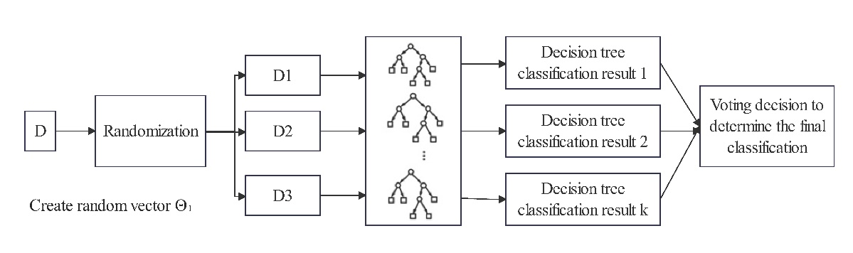
Figure 1: RF Diagram

Random Forest increases the diversity among classification models by constructing different training sets, thereby enhancing the extrapolation and predictive ability of the ensemble classification model. Through k rounds of training, a sequence of classification models \( \lbrace {h_{1}}(x),{h_{2}}(x),…,{h_{k}}(x)\rbrace \) is obtained, which together form a multi-classification model system. The final classification result of this system is determined by a simple majority voting method. The final classification decision is given by:

\( H(x)=arg\underset{y}{max}\sum _{i=1}^{k}I({h_{i}}(x)=y) \) (1)

where H(x) represents the combined classification model;

\( {h_{i}} \) denotes a single decision tree classification model;

\( y \) represents the output variable (or target variable);

\( I({h_{i}}(x)) \) is the indicator function.

Equation (1) illustrates the use of majority voting to determine the final classification.

3.2. Feature Extraction

Traditional signal features [11]-[13] commonly include time-domain and frequency-domain features. Time-domain features encompass mean value, variance, standard deviation, and peak value, while frequency-domain features include spectral energy, spectral entropy, and frequency. By reviewing extensive literature [6][16] and analyzing the trend changes in precursor feature signals, this paper introduces four new features: moving average slope, EWMA, EWMA rate of change, and percentage change. To smooth data while preserving necessary details, a sliding window technique is employed with a window size of 5. For each set of acoustic emission and electromagnetic radiation signal data, the sliding maximum, sliding minimum, sliding mean, sliding standard deviation, sliding spectral energy, sliding spectral entropy, moving average slope, EWMA, EWMA rate of change, and percentage change are calculated.

The calculation formulas for each parameter are as follows:

Sliding Maximum:

\( Max=max({x_{1}},{x_{2}},...,{x_{n}}) \) (2)

Sliding Minimum:

\( Min=min({x_{1}},{x_{2}},...,{x_{n}}) \) (3)

Sliding Mean:

\( Mean=\frac{1}{n}\sum _{i=1}^{n}{x_{i}} \) (4)

Sliding Standard Deviation:

\( SD=\sqrt[]{\frac{1}{n}\sum _{i=1}^{n}{({x_{i}}-Mean)^{2}}} \) (5)

where \( {x_{1}}, {x_{2}}, …, {x_{n}} \) represents the values within the sliding window, and \( n \) denotes the window size, which is 5.

Sliding Spectral Energy:

Calculated using Fourier Transform (FFT):

\( E=\sum _{k=1}^{N}{|X(k)|^{2}} \) (6)

where \( X(k) \) is the spectral amplitude at frequency k.

Sliding Spectral Entropy:

Calculated using Fourier Transform:

\( {P_{i}}=\frac{|X(i){|^{2}}}{\sum _{k=1}^{N}X(k){|^{2}}} \) (7)

where \( X(i) \) is the normalized spectral amplitude at frequency \( i \) .

Moving Average Slope:

Indicates the rate of change of the average value within a given window, helping to capture short-term signal trends:

\( {S_{t}}=\frac{ \sum _{i=0}^{n-1}i({y_{t-i}}-{\bar{y}_{t}})}{\sum _{i=0}^{n-1}{i^{2}}} \) (8)

where \( {y_{t}} \) is a time series, n is the window size, and \( {\bar{y}_{t}} \) is the average value within the window.

Exponentially Weighted Moving Average (EWMA):

Emphasizes recent observations for data smoothing and trend highlighting:

\( EWM{A_{t}}=α\cdot {y_{t}}+(1-α)\cdot EWM{A_{t-1}} \) (9)

where \( α \) is the smoothing constant, \( 0≤α≤1 \) , and \( {y_{t}} \) is the observation at time t.

EWMA Rate of Change ( \( ∆{Rate_{EWMA,t}} \) ):

Measures the rate of change of EWMA, reflecting the acceleration of signal changes:

\( ∆Rate(EWMA,t)=\frac{EWM{A_{t}}-EWM{A_{t-1}}}{EWM{A_{t-1}}} \) (10)

Percentage Change ( \( ∆{Rate_{EWMA,t}} \) ):

Describes the percentage change between data points in the time series, aiding in trend intensity identification:

\( ∆Rat{e_{per,t}}=\frac{{y_{t}}-{y_{t-1}}}{{y_{t-1}}}×100\% \) (11)

3.3. Feature Determination

Point biserial correlation analysis is a statistical method that can be used to study the relationship between two or more variables. It is primarily used to understand the strength and direction of the correlation or relationship between variables. After extracting the features of the signals, point biserial correlation analysis is employed to analyze the precursor feature signals, aiming to identify the time intervals of precursor features in electromagnetic radiation and acoustic emission signals.

The process for calculating the correlation between each feature parameter and the class is as follows:

Step 1: Calculate the means of the quantitative parameter \( \bar{X} \) and the dichotomous parameter \( \bar{Y} \) .

Step 2: Compute the deviation product for each data point between the quantitative parameter and the dichotomous parameter, and sum all the deviation products to get the total sum.

Step 3: Calculate the standard deviations of the quantitative parameter and the dichotomous parameter.

Step 4: Calculate the point biserial correlation coefficient.

The formula for calculating the point biserial correlation coefficient is as follows:

\( {r_{pd}}=\frac{∑({X_{i}}-\bar{X})×({Y_{i}}-\bar{Y})}{{S_{X}}×{S_{Y}}} \) (12)

where \( {X_{i}} \) and \( {Y_{i}} \) represent the values of the quantitative parameter and the dichotomous parameter for the \( i \) data point, respectively, and \( \bar{X} \) and \( \bar{Y} \) are the means of the two variables.

4. Case Analysis

4.1. Data Description and Data Processing

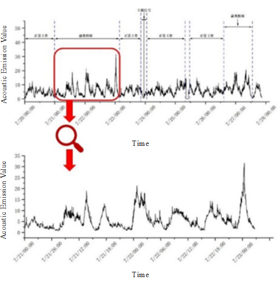
Figure 2: Amplitude Distribution Chart at the Time of Launch

Based on the data detected during actual production at a certain mining site, a dataset of acoustic emission signals and electromagnetic radiation signals was compiled. This data includes the statistical values of acoustic emission signal quantities and electromagnetic radiation signal quantities at different time periods during the production process, as well as the statistical classification of signal categories detected at different time periods. After feature extraction and processing, the following data was obtained.

The following table shows a portion of the AE data after preliminary organization and feature processing:

Table 1. Partially Processed AE Data Table after Feature Processing

The partially processed electromagnetic radiation signal data is shown in the following table:

Table 2. Partially Processed Electromagnetic Radiation Signal Data Table after Feature Processing

Step 1: Given Dataset

First, a dataset of acoustic emission signals and electromagnetic radiation signals is provided, which includes their feature values and target values. Based on the five features identified earlier, the selected feature values are the sliding mean, sliding standard deviation, sliding minimum, sliding maximum, and sliding spectral energy. The signal category is used as the target value, where interference signals are labeled as 1 and non-interference signals as 0.

Step 2: Data Preprocessing

Check the dataset for missing and abnormal values. Since the selected features are sliding parameters of the data within their respective windows and the sliding window size is set to 5, the last four rows of the dataset for both acoustic emission and electromagnetic radiation signals contain missing values. These rows should be removed.

Step 3: Splitting Training and Testing Sets

Divide 70% of the data into the training set and 30% into the testing set.

4.2. Feature Selection and Determination

Using point-biserial correlation analysis, it was found that for both electromagnetic radiation and acoustic emission signals, the five metrics—sliding mean, moving average slope, EWMA, EWMA change rate, and percentage change—show a strong correlation with precursor features. Therefore, these five metrics are selected as feature values for both electromagnetic radiation and acoustic emission signals. Consequently, the trend features of the data before the occurrence of danger for both electromagnetic radiation and acoustic emission signals are: sliding mean, moving average slope, EWMA, EWMA change rate, and percentage change.

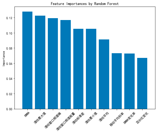
Figure 3: Feature Importance of Random Forest

4.3. Model Setup

Step 1: Constructing Decision Trees [7-10]:

Random forests are ensemble models consisting of multiple decision trees, so the first step is to construct these trees. A decision tree is a tree-like model used for classification or regression of instances. The construction process of a decision tree is recursive, involving the selection of the best features to split the dataset into different subsets until a stopping condition is met (such as reaching the maximum depth or having fewer samples than a certain threshold in a node).

Step 2: Random Feature Selection:

During the construction of each decision tree, a feature is selected from the set of all features for splitting. To introduce randomness, a subset of features is randomly selected at each node for consideration. This approach ensures that each tree is different, increasing randomness and enhancing the model’s generalization ability.

Step 3: Random Sampling of Data:

In building each decision tree, random sampling with replacement is typically performed on the training set to generate different subsets of training data. This method, known as “bootstrap sampling,” results in slightly different training datasets for each decision tree, increasing model diversity.

Step 4: Building Multiple Decision Trees:

To create a random forest model, multiple decision trees need to be built and combined to form a robust ensemble model. The number of trees to be constructed can be specified; in this case, we set the number of trees to 100. More trees generally improve the model’s stability and accuracy, but this needs to be balanced with computational cost and time.

Step 5: Voting by Decision Trees [17-18]:

When predicting for test samples, each decision tree provides a prediction result. The random forest model aggregates these results through voting to determine the final prediction. The calculation formula is as follows:

\( \hat{y}(x)=argma{x_{c}}\sum _{t-1}^{T}{P_{t}}(c|x) \) (13)

Among them, \( \hat{y}(x) \) represents the predicted category of sample \( x \) ;

\( argma{x_{c}} \) is the category with the highest summed probability;

\( {P_{t}}(c|x) \) denotes the probability that the \( t \) decision tree in the random forest predicts sample belongs to category \( c \) .

Step 6: Model Tuning

The random forest model has several important hyperparameters that need to be tuned, such as the number of decision trees, the maximum depth of each tree, and the minimum number of samples required at each node. In this step, we use cross-validation to select the optimal hyperparameter combination to enhance the model’s performance, ensuring that it maintains good predictive accuracy on unseen data.

Expressed mathematically:

\( RF(x)=mode(h({x_{2}}k))_{k=1}^{K} \) (14)

where \( X \) is the feature space; \( Y \) is the target variable (label); \( h(X, {Θ_{k}}) \) represents the prediction result of the sample by the \( k \) decision tree; \( {Θ_{k}} \) denotes the parameters of the \( k \) decision tree obtained through introducing randomness during the training process; “mode” refers to the majority voting mechanism, meaning the final classification result is determined by selecting the most frequent class label among all trees.

5. Model Solution and Results Explanation

Based on the importance indicators of various features mentioned above, we selected EWMA, sliding maximum, sliding window spectral entropy, sliding window spectral energy, and sliding standard deviation as the feature vectors. The signal class is used as the feature value (where precursor feature signals are labeled as 1 and non-precursor feature signals are labeled as 0). First, we employed down-sampling to balance the sizes of data labeled as 0 and 1. Subsequently, a random forest binary classification model was established, with the dataset split into training and testing sets for model training and evaluation. The resulting confusion matrix is shown below:

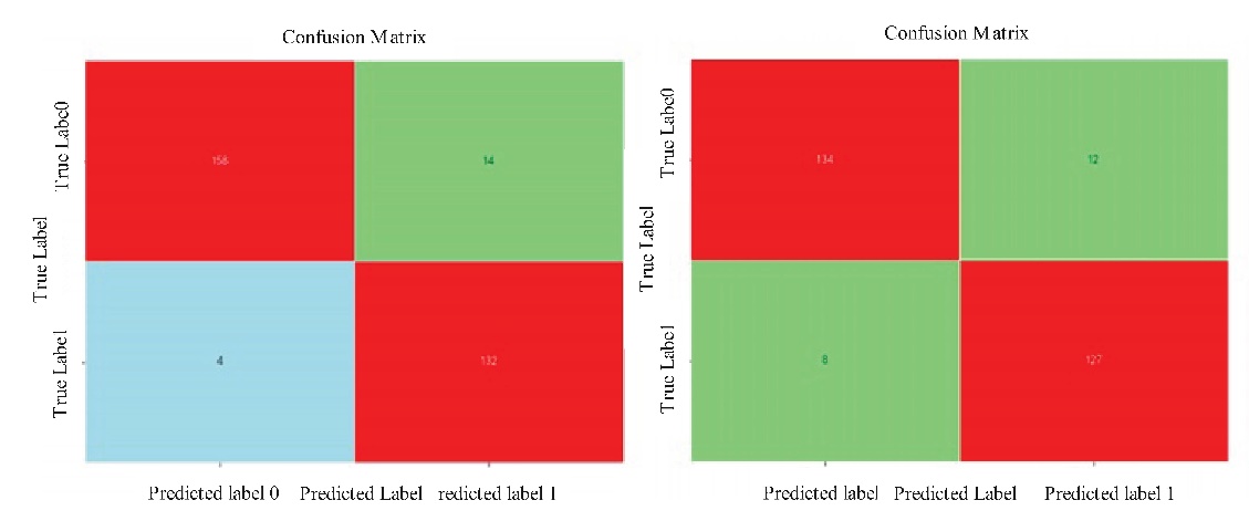
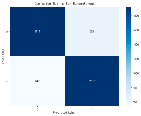
Figure 4: Confusion Matrix Chart

To demonstrate that our model has good accuracy and can correctly identify precursor feature signals, we set a continuous window size of 28 when using the model for signal identification. This measure ensures that only when the number of continuously predicted data points exceeds this window length will it be classified as a precursor feature signal. Using this method, we successfully identified the time intervals of the first five precursor feature signals in electromagnetic radiation and acoustic emission signals. The specific results are shown in the tables below:

Table 3. Time Intervals of Electromagnetic Radiation Precursors

Table 4. Time Intervals of Acoustic Emission Precursors

Based on the binary random forest model established above, the partial results are calculated as follows:

Table 5. Predicted and Actual Values of Acoustic Intensity Signals

Table 6. Predicted and Actual Values of Electromagnetic Radiation Signals

Prediction Results:

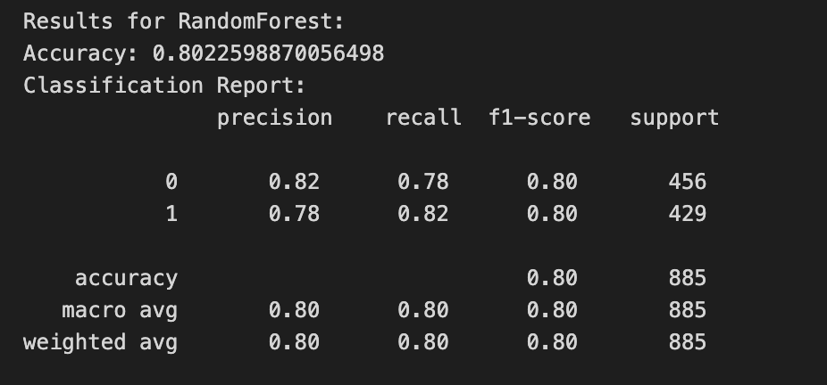
Figure 6: Prediction Results Chart

6. Conclusion

In summary, this paper proposes a signal recognition and prediction system based on the random forest model, applied to the hazard prediction of dynamic pressure in deep coal mining. Through the extraction and analysis of features from electromagnetic radiation (EMR) and acoustic emission (AE) signal data, we successfully constructed a random forest binary classification model to identify interference signals and precursor feature signals. To enhance the accuracy and reliability of predictions, we introduced new features such as moving average slope and exponential weighted moving average (EWMA), and employed down-sampling techniques to balance the data categories.

Overall, the proposed method not only effectively improves the accuracy of dynamic pressure prediction but also provides reliable data support for coal mine safety management. Future research could further optimize model parameters, explore additional factors affecting dynamic pressure, and validate the model’s applicability under different mining conditions to enhance the system’s generalization ability and practical value.

References

[1]. Wu, B. (2024). Study on the prediction model for dynamic pressure hazard based on supervised learning [Doctoral dissertation, Anhui University of Science and Technology].
[2]. Lu, C., et al. (2005). Spectrum analysis and signal recognition of rock mass microseismic monitoring. Journal of Geotechnical Engineering, 27(7), 772-775.
[3]. Zhou, X., He, X., & Zheng, C. (2019). Radio signal recognition based on deep learning in images. Journal on Communication/Tongxin Xuebao, 40(7).
[4]. Mai, Q., & Wu, X. (2024). Current status of coal mine dynamic pressure hazard prediction and monitoring technology. Shaanxi Coal, 43(01), 87-92.
[5]. Liang, Y., Shen, F., Xie, Z., et al. (2023). Research on dynamic pressure prediction method based on LSTM model. China Mining, 32(05), 88-95.
[6]. Di, Y. (2023). Research on comprehensive early warning for dynamic pressure based on deep learning [Doctoral dissertation, China University of Mining and Technology].
[7]. Fang, K., Wu, J., Zhu, J., et al. (2011). A review of random forest methods. Statistical & Information Forum, 26(03), 32-38.
[8]. Zhang, Z., et al. (2009). A review of radar radiation source signal recognition. Ship Electronic Engineering, 4, 10-14.
[9]. Rigatti, S. J. (2017). Random forest. Journal of Insurance Medicine, 47(1), 31-39.
[10]. Speiser, J. L., et al. (2019). A comparison of random forest variable selection methods for classification prediction modeling. Expert Systems with Applications, 134, 93-101.
[11]. Zhong, Z., & Li, H. (2020). Recognition and prediction of ground vibration signals based on machine learning algorithms. Neural Computing and Applications, 32(7), 1937-1947.
[12]. Zhao, D., & Yan, J. (2011). Performance prediction methodology based on pattern recognition. Signal Processing, 91(9), 2194-2203.
[13]. Keenan, R. J., et al. (2001). The signal recognition particle. Annual Review of Biochemistry, 70(1), 755-775.
[14]. Yuan, R., Li, H., & Li, H. (2012). Distribution characteristics and precursor information discrimination of coal pillar-type dynamic pressure microseismic signals. Journal of Rock Mechanics and Engineering, 31(01), 80-85.
[15]. Zhang, J., et al. (2019). An automatic recognition method of microseismic signals based on EEMD-SVD and ELM. Computers and Geosciences, 133, 104318.
[16]. Zhang, J., Jiang, R., Li, B., et al. (2019). An automatic recognition method of microseismic signals based on EEMD-SVD and ELM. Computers and Geosciences, 133, 104318.
[17]. Probst, P., & Boulesteix, A. L. (2018). To tune or not to tune the number of trees in random forest. Journal of Machine Learning Research, 18(181), 1-18.
[18]. Probst, P., Wright, M. N., & Boulesteix, A. L. (2019). Hyperparameters and tuning strategies for random forest. Wiley Interdisciplinary Reviews: Data Mining and Knowledge Discovery, 9(3), e1301.
Cite this article
Hu,J. (2024). Signal recognition and prediction system based on random forest model. Applied and Computational Engineering,95,68-78.
Data availability
The datasets used and/or analyzed during the current study will be available from the authors upon reasonable request.
Disclaimer/Publisher's Note
The statements, opinions and data contained in all publications are solely those of the individual author(s) and contributor(s) and not of EWA Publishing and/or the editor(s). EWA Publishing and/or the editor(s) disclaim responsibility for any injury to people or property resulting from any ideas, methods, instructions or products referred to in the content.
About volume
Volume title: Proceedings of the 6th International Conference on Computing and Data Science
© 2024 by the author(s). Licensee EWA Publishing, Oxford, UK. This article is an open access article distributed under the terms and
conditions of the Creative Commons Attribution (CC BY) license. Authors who
publish this series agree to the following terms:
1. Authors retain copyright and grant the series right of first publication with the work simultaneously licensed under a Creative Commons
Attribution License that allows others to share the work with an acknowledgment of the work's authorship and initial publication in this
series.
2. Authors are able to enter into separate, additional contractual arrangements for the non-exclusive distribution of the series's published
version of the work (e.g., post it to an institutional repository or publish it in a book), with an acknowledgment of its initial
publication in this series.
3. Authors are permitted and encouraged to post their work online (e.g., in institutional repositories or on their website) prior to and
during the submission process, as it can lead to productive exchanges, as well as earlier and greater citation of published work (See
Open access policy for details).