1.Introduction

As industrial and information technologies rapidly evolve, robots are widely used in high-risk, high-complexity industrial fields [1]. In order to improve work efficiency and reduce work risks, robots are increasingly deployed in extreme environments such as field surveys, planetary exploration, etc [2]. These complex and changeable environments place higher demands for the robot 's ground adaptability level, and thus we urgently need an effective method to classify the ground where the robot is located, so that the robot can accomplish tasks in different environments.

Common ground-based classification methods in the field can be categorized into traditional machine learning algorithms and deep learning algorithms based on neural networks. Tsai et al. [3] combined aerial radar data and photographic images to extract geometric features and spectral features, followed by a classification study of ground cover types using decision trees and support vector machines. Khairul Azmi Mahadhir et al. [4] used support vector machine (SVM) algorithm to identify different terrains by analyzing vibration signals, and then implement terrain classification for agricultural robots. Wenzhao Liao [5] used genetic algorithm to optimize the random forest model, and the optimized model has achieved a classification accuracy of 92.6%, which effectively improves the accuracy of ground classification. M. G. Harinarayanan Nampoothiri et al. [6] used machine learning techniques to develop a 100% accurate Ensemble-Subspace KNN based classification model, which can identify 11 terrain types for autonomous robots in real time. Although the machine learning algorithms can achieve good results, these algorithms usually need to manually design features, which is a tedious and difficult process, and it performs poorly when analyzing high-dimensional and complex ground data.

In recent years, with the improvement of arithmetic power and the development of artificial intelligence, scholars have begun to use neural-network-based deep learning approaches: Xinyun Zou et al. [7] proposed a reserve network (r-SNN) method based on spiking neuron networks for terrain classification using sensor data and camera images, and achieved an accuracy of more than 95 %. Amirreza Shaban et al. [8] employed a deep neural network called BEVNet for terrain classification, which can directly predict terrain classes of local maps from sparse LiDAR input data. Junghee Lee et al. [9] used convolutional neural network (CNN) as the main classification algorithm to convert one-dimensional spectral vectors into two-dimensional feature representations for ground cover classification studies. Ahmadreza Ahmadi et al. [10] used gated recurrent neural networks for semi-supervised robotic ground classification. Although deep learning algorithms can automatically learn the ground features, the deep learning algorithm applied by most scholars only processes in the time domain space and does not consider frequency domain features, which makes the network unable to capture the deep information behind the signal, making it difficult to make further breakthroughs in classification.

To tackle the above problems, this paper proposes a ground classification algorithm based on improved HHT algorithm based on EEMD and LSTM. The HHT algorithm is utilized to capture the frequency domain information in the signal that is difficult to be directly mined by the model. After that, the powerful feature extraction capability of the LSTM model is utilized for further learning and classification. This method can fully exploit the frequency domain features of the signal and take advantage of LSTM to achieve more accurate ground classification results.

2.Method

2.1.Hilbert-Huang transform

2.1.1.Empirical Modal Decomposition.

Hilbert-Huang Transform (HHT) can process nonlinear and non-stationary signals [11], which obtains the frequency domain information such as the instantaneous frequency of the signal and is very suitable for our signal data set. Specifically, the HHT contains two steps of empirical modal decomposition and Hilbert spectral analysis, where:

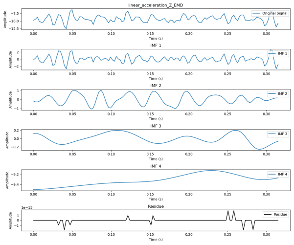
Empirical modal decomposition (EMD) is an adaptive method for analyzing time series data. It decomposes a complex time series into a series of intrinsic modal functions (IMFs), and then performs Hilbert transform on each IMF to extract features. However, the traditional EMD decomposition will produce problems such as modal aliasing and endpoint effects. Therefore, we use ensemble empirical modal decomposition (EEMD) to replace the traditional EMD to analyze the signals. EEMD adds noise several times and performs average processing on the basis of the EMD, so it can effectively avoid the modal aliasing problem of the EMD. Figure 1 shows the IMFs obtained by EMD decomposition of the input signal, and figure 2 shows the IMFs obtained by EEMD decomposition. It can be seen that the decomposition result of EEMD is more stable.

The procedure for EEMD decomposition is delineated as follows:

(1) Add N sets of white noise\( {n_{i}}(t) \)with standard normal distribution to the original input signal\( x(t) \)to obtain a new signal\( {x_{i}}(t) \):

\( {x_{i}}(t)=x(t)+{n_{i}}(t) \)(1)

(2) For the new signal\( {x_{i}}(t) \), EMD decomposition is performed to obtain J IMF components\( {c_{i,j}}(t) \)and residual function\( {r_{i}}(t) \):

\( {x_{i}}(t)=\sum _{j=1}^{J}{c_{i,j}}(t)+{r_{i}}(t) \)(2)

where\( {c_{i,j}}(t) \)is the j-th intrinsic mode function obtained by EMD decomposition of the new signal\( {x_{i}}(t) \), and\( {r_{i}}(t) \)is the residual function of the new signal\( {x_{i}}(t) \)obtained by the EMD decomposition .

(3) Perform an ensemble average operation on the aforesaid IMF components to achieve the final IMF of EEMD decomposition of the original input signal\( x(t) \):

\( {c_{j}}(t)=\frac{1}{N}\sum _{i=1}^{N}{c_{i,j}}(t) \)(3)

where\( {c_{j}}(t) \)is the j-th intrinsic mode function acquired through EEMD decomposition of the original input signal\( x(t) \).

Ultimately, the original input signal\( x(t) \)is represented by the following formula:

\( x(t)=\sum _{j=1}^{J}{c_{j}}(t)+r(t) \)(4)

2.1.2.Hilbert spectral analysis.

The original input signal\( x(t) \)is decomposed by EEMD to extract J intrinsic mode functions. Then, Hilbert transform is used for time-frequency analysis of each IMF component\( {c_{j}}(t) \), and the instantaneous frequency and instantaneous amplitude of the IMF are calculated to obtain the frequency domain characteristics of the signal.

The Hilbert transform of\( {c_{j}}(t) \)is defined as:

\( H[{c_{j}}(t)]={\hat{c}_{j}}(t)=\frac{1}{π}\int _{-∞}^{∞}\frac{{c_{j}}(t)}{t-τ}dτ \)(5)

After the Hilbert transform, the analytic signal corresponding to\( {c_{j}}(t) \)is defined as:

\( {z_{j}}(t)={c_{j}}(t)+i{c_{j}}(t)={a_{j}}(t)exp[i{θ_{j}}(t)] \)(6)

\( {a_{j}}(t)=[c_{j}^{2}(t)+\hat{c}_{j}^{2}(t){]^{1/2}} \)(7)

\( {θ_{j}}(t)=arctan\frac{{\hat{c}_{j}}(t)}{{c_{j}}(t)} \)(8)

\( {a_{j}}(t) \)is the envelope of the signal\( {z_{j}}(t) \), and\( {θ_{j}}(t) \)is the phase of the signal\( {z_{j}}(t) \).

The instantaneous frequency of\( {c_{j}}(t) \)is:

\( {ω_{j}}(t)=\frac{d{θ_{j}}(t)}{dt} \)(9)

Thus, the frequency domain characteristics of the input signal are obtained

Empirical modal decomposition (EMD) is an adaptive time series analysis method. It decomposes a complex time series into a series of intrinsic modal functions (IMFs), and then performs Hilbert transform on each

2.2.Long short-term memory networks

LSTM is a recurrent neural network with special structure and function, which controls the flow of information through input gates, forgetting gates, and output gates, so that LSTM can selectively retain or forget information, overcoming the gradient disappearance and gradient explosion problems faced by traditional RNNs, and being able to handle long sequence data more effectively¹². The input data set is 3810*128 long sequence data, which is suitable for LSTM model to process and complete the classification problem. Figure 3 illustrates the structure of the LSTM network.

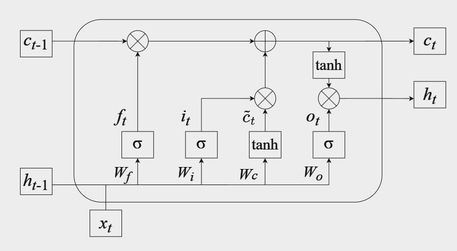
(1) Input gate controls which information from the current input should be stored in the cell state:

\( {i_{t}}=σ({W_{i}}\cdot [{h_{t-l}},{x_{t}}]+{b_{i}}) \)(10)

\( {\widetilde{c}_{t}}=tanh({W_{c}}\cdot [{h_{t-l}},{x_{t}}]+{b_{c}}) \)(11)

(2) Forget gate decides what information should be discarded from the cell state:

\( {f_{t}}=σ({W_{f}}\cdot [{h_{t-l}},{x_{t}}]+{b_{f}}) \)(12)

(3) Output gate controls what information about the cell state will be included in the next hidden state:

\( {o_{t}}=σ({W_{o}}\cdot [{h_{t-l}},{x_{t}}]+{b_{o}}) \)(13)

\( {h_{t}}={o_{t}}⊙tanh{(}{c_{t}}) \)(14)

(4) Cell state:

\( {c_{t}}={f_{t}}⊙{c_{t-l}}+{i_{t}}⊙{\widetilde{c}_{t}} \)(15)

In the above equation,\( {W_{i}}､{W_{c}}､{W_{f}}､{W_{o}} \)are the weight matrix, and\( {b_{i}}､{b_{c}}､{b_{f}}､{b_{o}} \)are the bias parameters, and\( σ \)is the sigmoid function, and\( ⊙ \)is the dot product.

3.Experiment

3.1.Experimental hardware and software environment

In this experiment, NVIDIA GeForce RTX 3060 is used as the GPU, Python version is 3.11.7. The neural network and model were constructed using the PyTorch 1.13.1 framework, which is developed in the PyCharm environment.

3.2.Dataset description

The data used in this experiment were obtained from¹³, the collector deployed 10 sensors in different ground environments for signal collection. Each set of signals collected by each sensor contains 128 sampling points, so each set of signals is a matrix with the shape of (128,10). Finally, 3810 sets of signal data were collected, and each set of data represents the characteristics of a specific ground type, which corresponds to 9 different ground types.

Figure 4 shows an example set of data collected by 10 sensors, and figure 5 shows the distribution of the nine different ground categories across all signals.

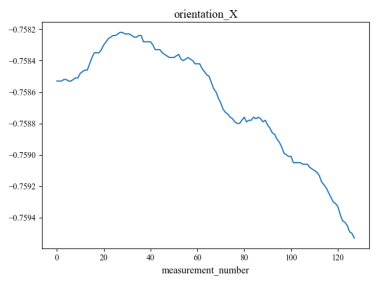
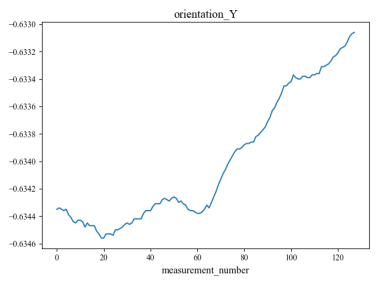
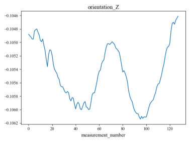
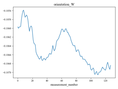
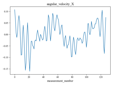
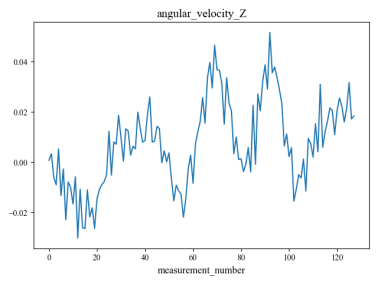
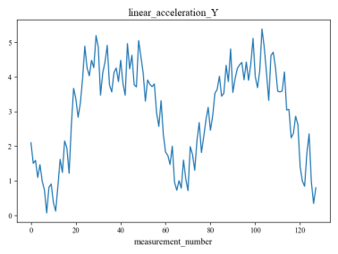
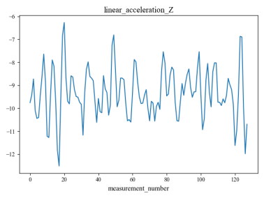
Figure 4. Waveforms of a set of signals acquired by 10 sensors.

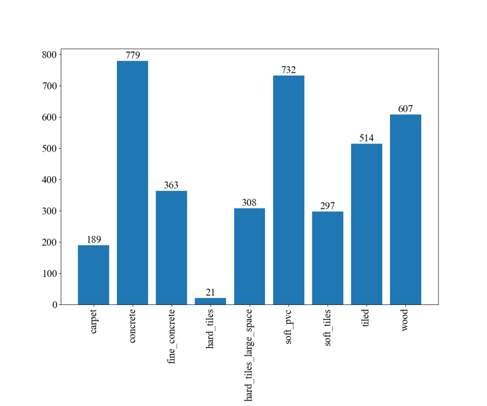
Figure 5. Distribution of ground categories.

3.3.Experimental Measurement Indicators

When using the neural network model for classification, we construct a 9*9 confusion matrix to assess the performance of the model. Each element in the confusion matrix\( {C_{ij}} \)represents the count of samples from class i that are categorized by the model as class j. The diagonal elements represent the count of samples accurately classified by the model, whereas the non-diagonal elements represent the number of samples misclassified. Based on the matrix, we can calculate the assessment indicators such as accuracy, precision, recall and F1 score in classification problems:

Accuracy measures the model's overall prediction efficacy by comparing the number of correct predictions to the total samples, as outlined in the following calculation:

\( Accuracy=\frac{\sum _{i=1}^{n}{C_{ii}}}{\sum _{i=1}^{n}\sum _{j=1}^{n}{C_{ij}}} \)(16)

Precision measures the ratio of all samples predicted to be positive by the model that are actually positive, reflecting the reliability of the model's predictive outcomes, as outlined below:

\( Precisio{n_{i}}=\frac{{C_{ii}}}{\sum _{j=1}^{n}{C_{ij}}} \)(17)

Recall measures the fraction of actual positive samples that are accurately classified as such by the model, reflecting the model's capacity to detect positive samples, and is computed as follows:

\( Recal{l_{i}}=\frac{{C_{ii}}}{\sum _{j=1}^{n}{C_{ji}}} \)(18)

The F1 Score (F1 Score) is the reconciled average of the precision and recall, which is employed to evaluate the balance of accuracy and completeness of the model. The computation formula is delineated below:

\( F{1_{i}}=2×\frac{Precisio{n_{i}}×Recal{l_{i}}}{Precisio{n_{i}}+Recal{l_{i}}} \)(19)

3.4.Comparative experiments

3.4.1.Comparison of classification models.

In order to select the final neural network model for classification, we compared the classification effects of LSTM and 1DCNN models. To ensure a fair comparison, we used the original data as the base dataset, trained and tested with the two models separately, and used the five-fold cross-validation method for metrics measurement. The cross-validation outcomes are delineated in table 1.

Table 1. Metrics for evaluating the LSTM model and 1DCNN model with five-fold cross-validation.

Table 1 illustrates that the precision of the LSTM model outperforms the 1DCNN model in classification tasks, so we selected LSTM as our classification model in the subsequent experiments.

3.4.2.Comparison of Empirical Modal Decomposition Methods

In the previous section, we mentioned that the decomposition of HHT transform has two different ways, EMD and EEMD, and the latter is an improvement of the former. In order to verify the different effects of the two approaches, we keep the rest of the conditions unchanged, and compare classification effect after decomposing dataset with EMD and EEMD respectively. The five-fold cross-validation is still adopted, and table 2 shows the classification results.

Table 2. Classification results corresponding to EMD and EEMD decomposition.

Table 2 shows that the average accuracy of EEMD is higher than that of EMD, which proves the effectiveness of EEMD as an improvement.

3.5.Ablation experiments

To evaluate the improvement effect of the HHT transform on the classification performance, we conducted classification experiments on the dataset containing only the original signals and the expanded dataset with the transformed signals respectively, while keeping all other conditions constant. The cross-validated results are shown in figure 6. The figure illustrates that our proposed HHT method can improve the classification accuracy, proving the effectiveness of our method.

4.Conclusion

Employing the dataset on the Kaggle website as the experimental dataset, this paper proposes a robot ground classification algorithm that combines EEMD and LSTM, which effectively realizes efficient classification of complex ground environments. The original dataset was collected by 10 sensors, containing a total of 3810 sets of signals and 9 ground types, and each set of signals is a matrix of size (128, 10). We conducted two sets of comparison experiments between EMD/EEMD and LSTM/1DCNN: the classification accuracy obtained using the original dataset combined with the LSTM model is 77.77%, while the classification accuracy using the improved HHT combined with EEMD algorithm and the LSTM model is improved to 79.32%, which proves the effectiveness of the EEMD improvement; the classification accuracy of the improved HHT combined with EEMD algorithm and 1DCNN model is only 38.40%, proving that LSTM is more suitable than 1DCNN for the task in this dataset. Additionally we performed ablation experiments to demonstrate the improvement and enhancement of the HHT transform for the results. Future work can further optimize the robot ground classification problem from the perspective of combining multiple deep learning methods and optimizing data processing for a wider range of application scenarios and higher robustness.

References

[1]. Wong C, Yang E, Yan XT, Gu D. Autonomous robots for harsh environments: a holistic overview of current solutions and ongoing challenges. Syst Sci Control Eng. 2018 Jan 1;6(1):213–9.
[2]. Chai H, Li Y, Song R, Zhang G, Zhang Q, Liu S, et al. A survey of the development of quadruped robots: Joint configuration, dynamic locomotion control method and mobile manipulation approach. Biomim Intell Robot. 2022 Mar;2(1):100029.
[3]. Tsai MD, Tseng KW, Lai CC, Wei CT, Cheng KF. Exploring Airborne LiDAR and Aerial Photographs Using Machine Learning for Land Cover Classification. Remote Sens. 2023 Apr 26;15(9):2280.
[4]. Mahadhir KA, Tan SC, Low CY, Dumitrescu R, Amin ATM, Jaffar A. Terrain Classification for Track-driven Agricultural Robots. Procedia Technol. 2014;15:775–82.
[5]. Liao W. Ground classification based on optimal random forest model. In: 2023 IEEE International Conference on Control, Electronics and Computer Technology (ICCECT) [Internet]. Jilin, China: IEEE; 2023 [cited 2024 May 7]. p. 709–14. Available from: https://ieeexplore.ieee.org/document/10141122/
[6]. Nampoothiri MGH, Anand PSG, Antony R. Real time terrain identification of autonomous robots using machine learning. Int J Intell Robot Appl. 2020 Sep;4(3):265–77.
[7]. Zou X, Hwu T, Krichmar J, Neftci E. Terrain Classification with a Reservoir-Based Network of Spiking Neurons. In: 2020 IEEE International Symposium on Circuits and Systems (ISCAS) [Internet]. 2020 [cited 2024 Apr 30]. p. 1–5. Available from: https://ieeexplore.ieee.org/abstract/document/9180740
[8]. Shaban A, Meng X, Lee J, Boots B, Fox D. Semantic Terrain Classification for Off-Road Autonomous Driving.
[9]. Lee J, Han D, Shin M, Im J, Lee J, Quackenbush LJ. Different Spectral Domain Transformation for Land Cover Classification Using Convolutional Neural Networks with Multi-Temporal Satellite Imagery. Remote Sens. 2020 Mar 30;12(7):1097.
[10]. Ahmadi A, Nygaard T, Kottege N, Howard D, Hudson N. Semi-Supervised Gated Recurrent Neural Networks for Robotic Terrain Classification. IEEE Robot Autom Lett. 2021 Apr;6(2):1848–55.
[11]. Ma C, Xie S, Bi CW, Zhao YP. Nonlinear dynamic analysis of aquaculture platforms in irregular waves based on Hilbert–Huang transform. J Fluids Struct. 2023 Feb;117:103831.
[12]. Guan Y, Liu J. Research on the Method of Remaining Useful Life Prediction of Lithium-ion Battery Based on LSTM. In: 2021 3rd International Conference on Advances in Computer Technology, Information Science and Communication (CTISC) [Internet]. Shanghai, China: IEEE; 2021 [cited 2024 Jun 29]. p. 226–31. Available from: https://ieeexplore.ieee.org/document/9527645/
[13]. CareerCon 2019 - Help Navigate Robots [Internet]. [cited 2024 Jul 7]. Available from: https://kaggle.com/competitions/career-con-2019
Cite this article
Guo,Z. (2024). Robot terrain classification based on improved Hilbert-Huang transform and long short-term memory network. Applied and Computational Engineering,95,49-56.
Data availability
The datasets used and/or analyzed during the current study will be available from the authors upon reasonable request.
Disclaimer/Publisher's Note
The statements, opinions and data contained in all publications are solely those of the individual author(s) and contributor(s) and not of EWA Publishing and/or the editor(s). EWA Publishing and/or the editor(s) disclaim responsibility for any injury to people or property resulting from any ideas, methods, instructions or products referred to in the content.
About volume
Volume title: Proceedings of the 6th International Conference on Computing and Data Science
© 2024 by the author(s). Licensee EWA Publishing, Oxford, UK. This article is an open access article distributed under the terms and
conditions of the Creative Commons Attribution (CC BY) license. Authors who
publish this series agree to the following terms:
1. Authors retain copyright and grant the series right of first publication with the work simultaneously licensed under a Creative Commons
Attribution License that allows others to share the work with an acknowledgment of the work's authorship and initial publication in this
series.
2. Authors are able to enter into separate, additional contractual arrangements for the non-exclusive distribution of the series's published
version of the work (e.g., post it to an institutional repository or publish it in a book), with an acknowledgment of its initial
publication in this series.
3. Authors are permitted and encouraged to post their work online (e.g., in institutional repositories or on their website) prior to and
during the submission process, as it can lead to productive exchanges, as well as earlier and greater citation of published work (See
Open access policy for details).