1.Introduction

In the rapid development of modern cities, fresh produce superstores have become an important part of the daily life of urban residents. As the main channel for providing fresh vegetables, fruits and other essential foods, fresh produce superstores play a crucial role in safeguarding the dietary health of urban residents. As people continue to pursue food quality and quality of life, the market demand for fresh produce continues to grow. However, there are quite a few challenges hidden behind this trend, especially in the supply chain management of vegetables. As one of the most common fresh products, vegetables are characterised by a high diversity of categories, a short shelf life and a fast sales cycle. These characteristics complicate vegetable supply chain management and make it a difficult task for fresh produce superstores to sell and replenish vegetables effectively.

Firstly, vegetables have a short shelf-life and are susceptible to environmental influences, and any small negligence in the process can lead to significant losses. This requires supermarkets to handle each batch of vegetables with great care, from procurement, transport, storage to display, all requiring strict quality control. Secondly, seasonal changes in vegetable sales bring another layer of complexity to supermarkets' purchasing decisions. Different vegetable categories have significant differences in their adaptability to climate, which directly affects their growth cycle and market supply. During different seasons, certain vegetables may be in abundant supply and inexpensive, while other varieties may be scarce and expensive. Supermarkets need to adjust their replenishment strategies according to these seasonal variations in order to maintain the diversity and freshness of the items on their shelves. Further, the inter-relationship between vegetable categories is an important factor to consider. There may be alternative or complementary selling relationships between certain vegetables. For example, if there is a shortage of one type of leafy vegetable, consumers may switch to other types of leafy vegetables. Understanding the interactions between these vegetables can help supermarkets better predict consumer behaviour and thus make more accurate replenishment decisions. In addition, the uncertainty of the price of incoming vegetables adds to the difficulty of supply chain management. Due to a variety of factors such as weather, transport costs, and market supply and demand, the purchase price of vegetables may fluctuate significantly. This poses a challenge to the cost control and pricing strategies of supermarkets and directly affects their profitability.

In view of the above challenges, the research objective is to analyse vegetable sales data in depth and explore the sales volume distribution patterns, seasonal variations and their interrelationships among different categories. Through a detailed study of historical sales data and wastage rates, the thesis hope to provide fresh produce superstores with insights that will help them improve their replenishment decisions and pricing strategies. Specifically, the thesis plan to apply statistical and data analysis methods to seasonally disaggregate the sales records of various vegetables in order to identify and predict sales trends within different seasons or time periods [1]. In addition, by exploring the correlation between vegetable categories, the thesis expect to identify potential substitution or complementary effects, which will provide a basis for superstores to optimise their vegetable assortment mix [2].

Through the above research, the thesis aim to provide scientific, data-driven management advice to fresh food superstores to help them cope with changing market demands and supply chain challenges. the thesis believe that by improving sales efficiency, reducing wastage, and ultimately providing more quality food to consumers, it can add competitiveness to the fresh produce superstore business and achieve sustainable growth. Ensuring the success of this study requires not only deep industry understanding and efficient data analysis techniques, but also the ability to closely integrate with actual marketing strategies. The thesis plan to work closely with the industry partners to ensure the practical application of the findings [3]. Ultimately, the thesis expect this study to help fresh produce superstores navigate the complex and dynamic market environment, and assist them in making solid strides in safeguarding food safety and improving consumer satisfaction [4].

2.Preliminary Analysis of Data

2.1.Descriptive statistical analysis of data

The thesis have six vegetable categories of product information and sales flow detail data, through the two tables of data merging and data preprocessing, eliminating outliers (sales of negative rows), missing values interpolation to 0, filtering out the sales of data to remove the return data [5].

The sales volume of each category of vegetables is counted on a monthly basis and the following table is obtained:

Table 1. Monthly sales volume of vegetables by category.

2.2.Distribution patterns and interrelationships of sales volume of vegetables by category

Firstly, Matlab was used to visually represent the monthly sales volume of each category of vegetables for 36 months and the following line and scatter plots were obtained:

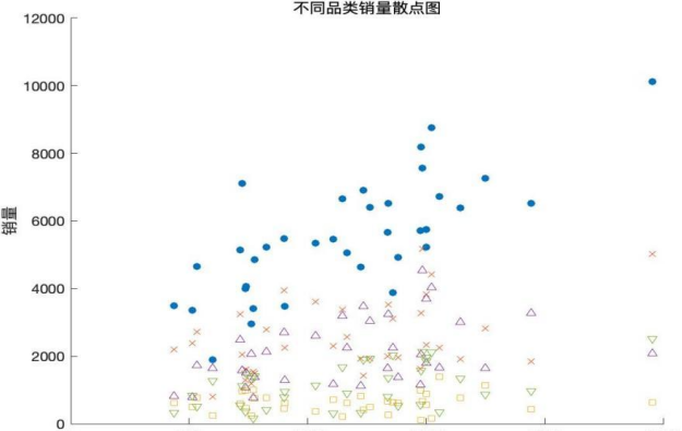
Figure 1: Scatterplot of monthly sales volume of vegetables by category for 36 months.

From the figure, it can be seen that the monthly sales of certain categories have the same fluctuation with the change of month, and the sales of certain categories are correlated with each other, and so carries out the correlation coefficient analysis for the correlation of the sales of categories with each other.

Correlation coefficient analysis:

First make a heat map for visualisation and then construct a matrix of correlation coefficients.

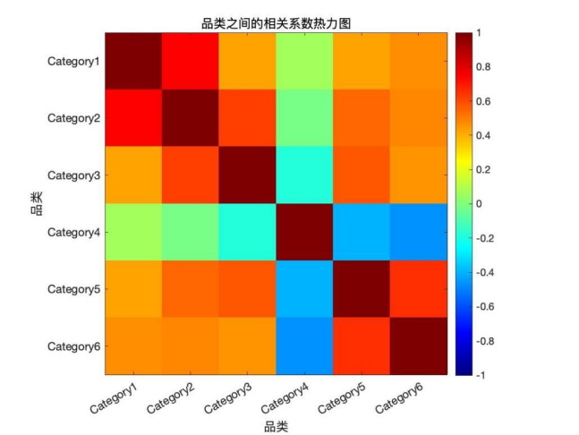
Figure 2: Heat Map of Seasonal Analysis of Sales Volume of Vegetables by Category.

Table 2.Correlation coefficient matrix.

It can be seen that there is a high degree of correlation between sales of foliar and flowering stem categories, and a weak negative trend for eggplant and aquatic rhizomes.

3.Optimal Solutions for Profit Maximisation in Each Vegetable Category

3.1.Relationship between total sales and "cost-plus pricing" for each vegetable category

First of all, the total sales of each vegetable category, from the background information, the thesis can know that "cost-plus pricing" refers to the commodity pricing, and then statistics on the pricing of each vegetable category, the use of random forest regression model, the construction of the decision tree is still based on the recursive partitioning nodes, usually use the following formula to select the best segmentation features decision tree construction based on the The decision tree is constructed based on the recursive segmentation nodes, and the following formula is usually used to select the best segmentation features[7].

Gini(D)=1-\( \sum _{K=1}^{K}(PK)² \)

Entropy(D)=-\( \sum _{K=1}^{K}PK{log_{2}}{PK} \)

With this algorithm, a plot of the relationship between total sales and pricing is obtained for each vegetable category (Y represents total sales and X represents pricing)

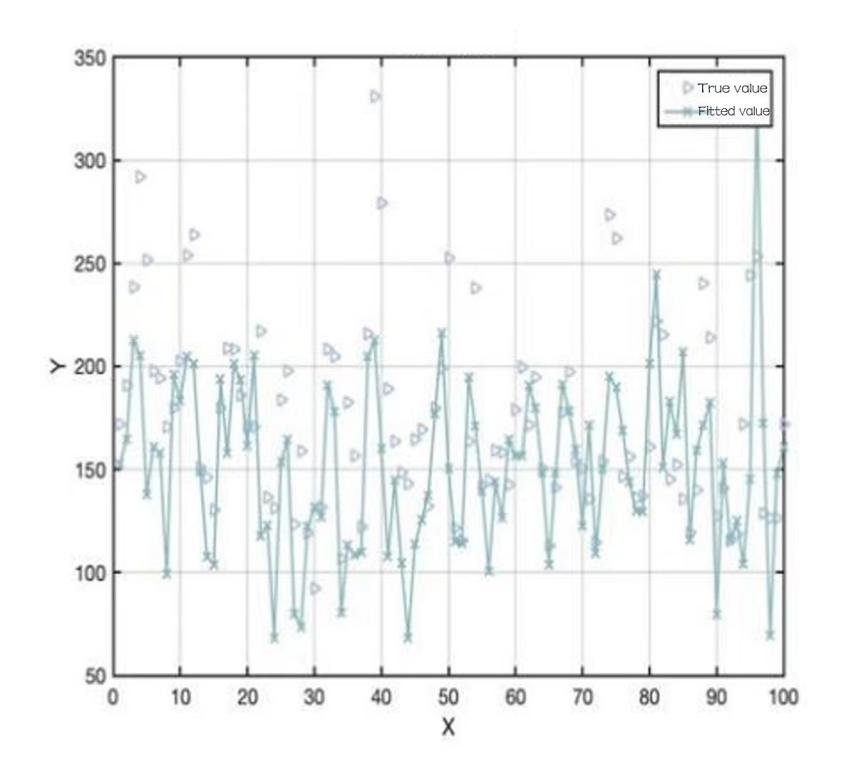
Figure 3: Total sales and pricing of mosaic vegetables.

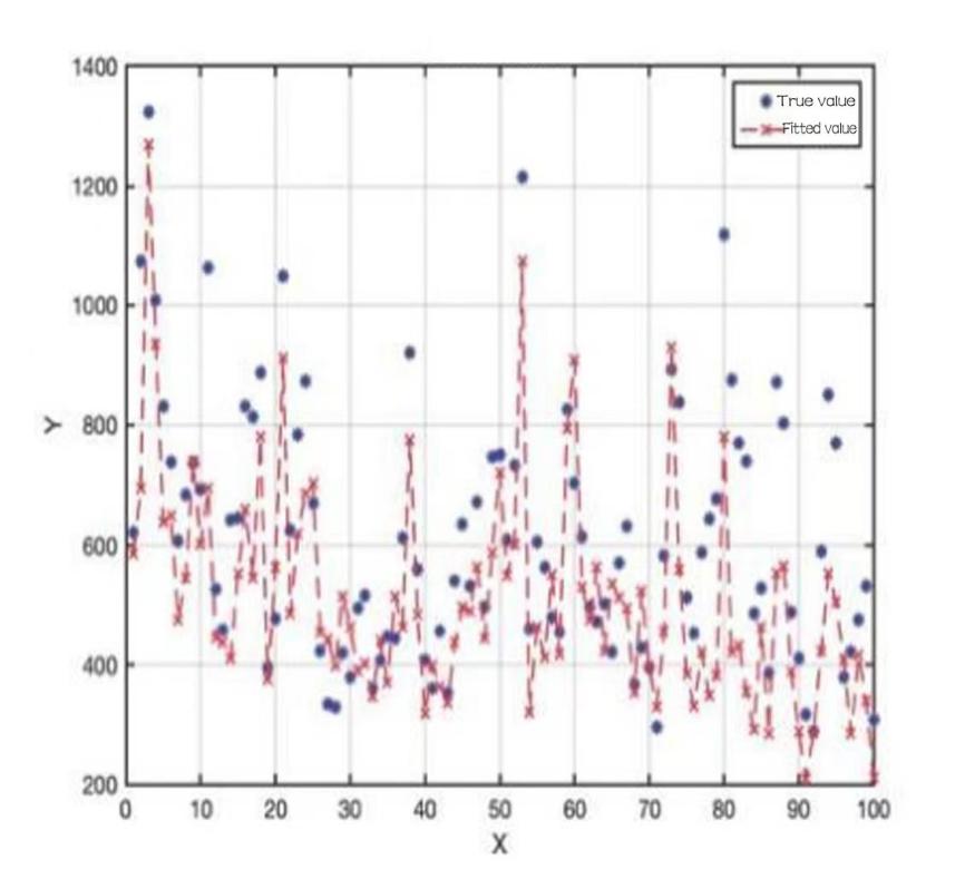
Figure 4: Total sales and pricing of cauliflower vegetables.

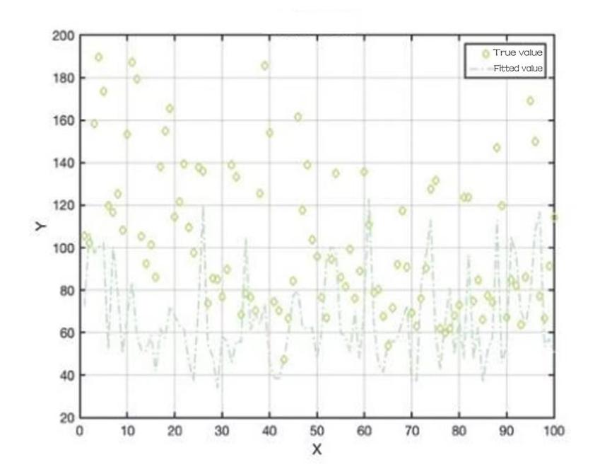
Figure 5: Total sales and pricing of pepper vegetables.

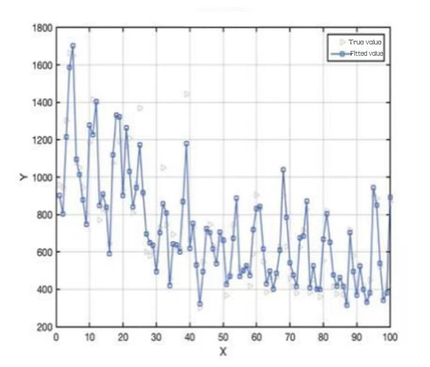
Figure 6: Total sales and pricing of edible mushroom vegetables.

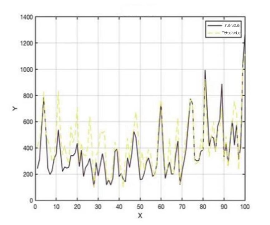
Figure 7: Total sales and pricing of aquatic root vegetables.

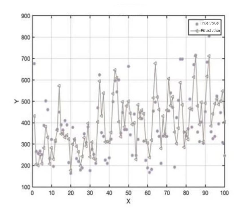
Figure 8: Total sales and pricing of nightshade vegetables.

Observation of the relationship between X and Y shows that the total sales of vegetable category has a weak negative relationship with cost plus pricing, based on this pattern, it helps to formulate the sales strategy accordingly.

3.2.Forecast of total daily replenishment for each vegetable category for the coming week

To predict the total daily replenishment for the coming week firstly the total daily sales for the coming week is predicted then the corresponding wastage rate is considered. The data for July 2020-2022 and June 2023 are selected and aggregated to predict the total sales for the coming week using the LSTM time series model, and then the LSTM time series model is optimised using the White Shark optimisation algorithm [8].

The formula for calculating the amount of incoming goods:

U=S×(1+K%)

It is possible to obtain a graph of the predicted sales of each type of vegetable dish:

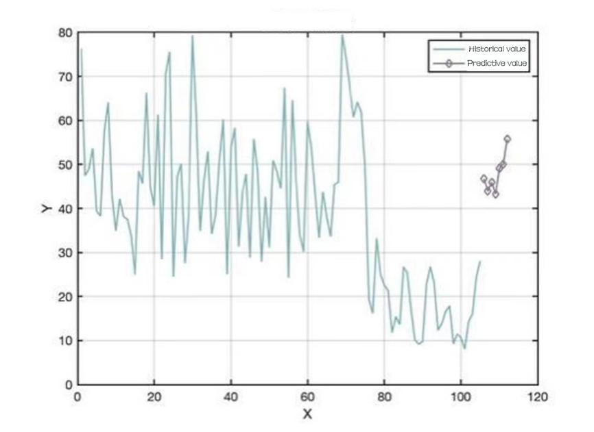
Figure 9: Sales of mosaic vegetables for the week ahead.

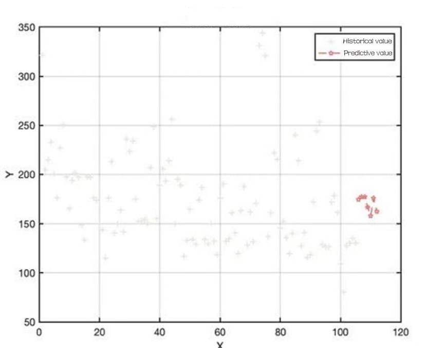
Figure 10: Sales of cauliflower vegetables for the week ahead.

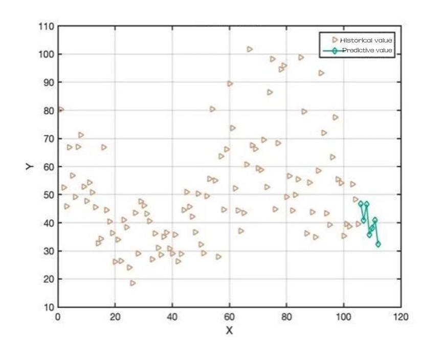
Figure 11: Sales of edible mushroom vegetables for the week ahead.

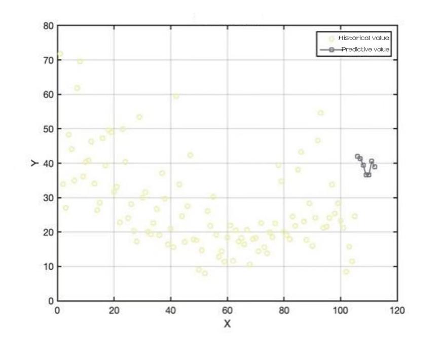
Figure 12: Sales of nightshade vegetables for the week ahead.

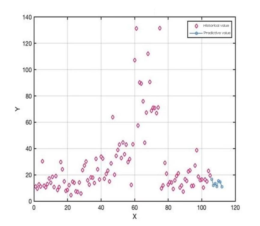
Figure 13: Sales of aquatic root vegetables for the week ahead.

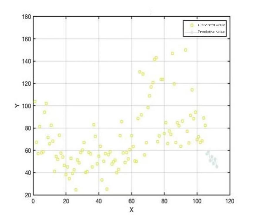
Figure 14: Sales of pepper vegetables in the week ahead.

The total daily replenishment for each vegetable category for the coming week can be calculated as shown in the table below:

Table 3. Total daily replenishment by vegetable category for the coming week.

3.3.Quantitative fitting of indicators for the vegetable category

Table 4. Monthly distribution of sales volume by category.

Table 5. Trend of profit distribution by category by month.

Table 6. Monthly trends in post-discount profits by category.

Table 7. Monthly distribution of post-discount sales volume by category.

3.4.Daily pricing strategy for each vegetable category for the week ahead

Based on the above data, a dynamic programming model is constructed to maximise the seven-day total profit W of the superstore, where the profit can be divided into normal sales profit and discount sales profit [9][10]. The specific modelling process is as follows:

(1) Decision variable: Quantitative polynomial fitting formula for each indicator in the vegetable category

(2) Objective function: Maximise profit of superstores

W=P×N×(1-K%)+P\( × \)N\( × \)(1-K%)

(3) restrictive condition

Constraint 1: Discount margin P usually has an upper and lower limit to ensure that the price is reasonable.

Constraint 2: Non-discounted profit P-runs usually have an upper and lower limit to ensure that they are reasonably priced.

Constraint 3: positive loss rate k per cent

Constraint 4: Non-discounted sales in each category N is restricted

Constraint 5: Discounted sales in each category N is restricted

Global optimal solution using particle swarm algorithm (PSO)

The optimal solution for pricing of each dish category is calculated using Matlab as shown in the table below:

Table 8. Optimal solution for pricing each dish.

4.Impact Of Other Fators On Sales Volume

4.1.Holiday factors

By filtering out the holidays: New Year's Day (1 day off on 1 January), Spring Festival (3 days off from the first to the third day of the first month of the lunar calendar), Qingming Festival (1 day off on the same day as Qingming on the lunar calendar), Labour Day (1 day off on 1 May), Dragon Boat Festival (1 day off on the same day as Dragon Boat Festival on the lunar calendar), Mid-Autumn Festival (1 day off on the same day as Mid-Autumn Festival on the lunar calendar), and National Day (3 days off on the 1st to the 3rd day of the 10th October), and comparing them with the average of the usual sales, as shown below:

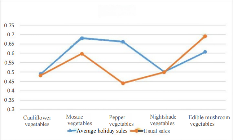
Figure 15: Comparison of holiday sales with usual sales.

It can be seen that the average holiday sales of each category are generally higher than the usual sales, and the average holiday sales of the chilli category are significantly higher than the usual sales, indicating that people generally love to eat heavy vegetables such as chilli during holidays. From this, it is a good way to go to restaurants, food markets and other places to collect data related to the sales volume of chilli.

4.2.Weather factors

Vegetable price volatility affects supply chains and consumer choice. Adverse weather can lead to reduced yields, increase storage and transport difficulties, and affect consumer demand. Traders have to make pricing decisions taking into account costs, changes in market demand and the impact of seasonality.

1. Availability: Weather conditions (e.g., droughts, floods, storms) affect vegetable production and may lead to price increases. Changes in production costs and changes in market demand need to be factored into pricing considerations.

2. Storage and transport: Certain vegetables require special handling to maintain quality and freshness. Adverse weather can damage the supply chain and make storage and transport more difficult, leading to unstable supplies and higher costs.

3. Consumer demand: Different weather conditions affect consumer demand for different types of vegetables. Summer may favour cool, water-rich vegetables, while winter requires high-energy, high-calorie vegetables. Traders should adjust their replenishment and pricing strategies according to seasonal demand.

5.Summary

This paper provides scientific management suggestions for fresh produce superstores through the study of vegetable sales and replenishment forecasting, using data integration, descriptive statistics and correlation analysis. The research results show that vegetable sales volume by month is more suitable for correlation analysis, and the sales volume of each category has a weak negative correlation with pricing. By building a prediction model, the daily replenishment volume in the coming week can be effectively predicted and profit can be improved with the help of optimisation algorithms. These findings are crucial for fresh produce superstores to navigate through the market environment and improve consumer satisfaction [11].

This study aims to provide scientific, data-driven management recommendations for fresh produce superstores to help address market demand and supply chain challenges. By improving sales efficiency, reducing wastage, and ultimately providing more quality food, fresh produce superstores can enhance their competitiveness and achieve sustainable growth. In addition, successful implementation of this study requires not only deep industry understanding and efficient data analysis techniques, but also close integration with actual marketing strategies. The team plan to work closely with the industry partners to ensure that the results of the study can be effectively applied. The team look forward to helping fresh produce superstores navigate the complex market environment through this study, helping them to safeguard food safety and enhance consumer satisfaction[12].

References

[1]. Tang Guosheng. Exploration on the Construction of Innovative Practice Base of Mathematical Modelling for College Students Based on SWOT Analysis--Taking Jiangsu University of Science and Technology as an Example[J]. Journal of Higher Education, 2023, 9(11): 53-56. DOI: 10. 19980/j.CN23- 1593/G4.2023.11.013.
[2]. Xie Yujing,Han Huili. A multidimensional analysis of mathematical modelling in the junior high school mathematics textbook of Bei Shi Da edition[J]. Teaching and Management, 2023(09):73-76.
[3]. LIU Zhimei. The deep integration of mathematical modelling and higher vocational mathematics teaching[J]. Journal of Jiamusi Vocational College,2023,39(03):152-154.
[4]. Xu Yatao,Wu Libao. Research on the evaluation index system of teaching mathematical modelling in high school based on Delphi-AHP[J]. Journal of Neijiang Normal College,2023,38(02):113-119.DOI:10.13603/j.cnki.51- 1621/z.2023.02.018.
[5]. YANG Benzhao, SHI Yanan, DUAN Qianheng, LI Guangsong, YU Gang. Exploration of full-cycle teaching practice for university students' mathematical modelling competition[J]. University Education,2023(04):44-46.
[6]. Huang Jian,Xu Binyan. Development trend of teaching and learning research on mathematical modelling in international perspective - an analysis based on the 14th International Congress on Mathematics Education[J]. Journal of Mathematics Education,2023,32(01):93-98.
[7]. Li Shuai. Research on commodity pricing and ordering strategy considering strategic buying behaviour in e-commerce environment[D]. Yanshan University,2018.
[8]. Hong Qihan. Optimal design of antenna based on improved simulated annealing and white shark algorithm[D]. Donghua University,2023.DOI:10.27012/d.cnki.gdhuu.2023.001164.
[9]. Braik M,Hammouri A,Atwan J,et al. White Shark Optimizer:A novel bio-inspired meta-heuristic algorithm for global optimisation problems[J]. Knowledge-Based Systems, 2022,243:108457.
[10]. Zeng, Minmin. Research on Dynamic Pricing Strategy of Fresh Community Supermarket Based on Time Situation A[D]. Southwest University of Finance and Economics, 2021. DOI:10.27412/d.cnki.gxncu.2021.002858.
[11]. Zhang He. Vegetable sales prediction based on integrated learning[D]. Yunnan Normal University,2021.DOI:10.27459/d.cnki.gynfc.2021.000144.
[12]. MENG Fanrong,ZHANG Peng,YAN Qiuyan. A data flow prediction model based on weighted moving average[J]. Computer Application Research,2009,26(10):3680-3682+3686.
Cite this article
Cai,M. (2024). Automated pricing and replenishment forecasting for vegetable items. Applied and Computational Engineering,95,34-48.
Data availability
The datasets used and/or analyzed during the current study will be available from the authors upon reasonable request.
Disclaimer/Publisher's Note
The statements, opinions and data contained in all publications are solely those of the individual author(s) and contributor(s) and not of EWA Publishing and/or the editor(s). EWA Publishing and/or the editor(s) disclaim responsibility for any injury to people or property resulting from any ideas, methods, instructions or products referred to in the content.
About volume
Volume title: Proceedings of the 6th International Conference on Computing and Data Science
© 2024 by the author(s). Licensee EWA Publishing, Oxford, UK. This article is an open access article distributed under the terms and
conditions of the Creative Commons Attribution (CC BY) license. Authors who
publish this series agree to the following terms:
1. Authors retain copyright and grant the series right of first publication with the work simultaneously licensed under a Creative Commons
Attribution License that allows others to share the work with an acknowledgment of the work's authorship and initial publication in this
series.
2. Authors are able to enter into separate, additional contractual arrangements for the non-exclusive distribution of the series's published
version of the work (e.g., post it to an institutional repository or publish it in a book), with an acknowledgment of its initial
publication in this series.
3. Authors are permitted and encouraged to post their work online (e.g., in institutional repositories or on their website) prior to and
during the submission process, as it can lead to productive exchanges, as well as earlier and greater citation of published work (See
Open access policy for details).