1. Introduction

1.1. Research background and significance

With the rapid development of the world's industrialization, the carbon content in the air continues to rise, leading to the melting of global two-stage glaciers, destroying the habitat of a large number of animals, and intensifying the greenhouse effect. The following figure shows the carbon dioxide emissions released by the world's environmental organizations in recent years[1,2].

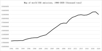
Figure 1. World carbon dioxide emissions

As can be seen from Figure 1, global carbon dioxide emissions have shown an overall upward trend since 1990. Under the influence of high carbon dioxide emissions over the years, the amount of carbon dioxide in the air has increased significantly[3]. In order to monitor changes in the amount of carbon dioxide in the air, accurate prediction of carbon dioxide levels has become essential.

1.2. Literature review

Wu Haijie [4]et al. predicted the carbon emission in the power system by using the grey BP neural network model, and the experiment showed that the grey BP neural network model had better effect than other prediction models. Zhang Lili[5]et al. introduced multiple prediction models and time series prediction models for the prediction of carbon dioxide concentration, and the prediction results showed that the time series prediction model was more accurate than the multiple prediction model in the prediction of carbon dioxide concentration. Swetha P S[6]et al. predicted carbon dioxide content through machine learning models such as random forest and found that the coefficient of determination calculated by random forest algorithm was higher than that of most machine learning algorithms.

In the past research on carbon dioxide emission prediction, most of them are limited to a single machine learning model, but the disadvantages of a single machine learning algorithm are obvious, such as the slow running speed of XGBoost algorithm and the inability of linear support vector machine to accurately fit the results. The prediction algorithms of multiple machine learning fusion models can greatly improve the goodness of fit of models and aggregate the advantages of multiple models compared with a single model. Therefore, this paper will fuse multiple base models and compare the prediction results of the base models to obtain a model for predicting future atmospheric carbon emissions in Europe.

2. Data preprocessing

This paper mainly collects data on carbon content in the air over the Alps. Due to the huge amount of data, some outliers are generated, including data beyond the theoretical range and some missing data. Therefore, it is necessary to conduct normality test and visualization of the data. When the sample data exceeds three times the standard deviation of the mean value, the data is judged as abnormal data. In order to ensure the integrity of the data, this paper uses linear interpolation to replace or supplement the outliers.

At the same time, in order to eliminate the negative effects brought by different dimensions, the data is normalized. The calculation formula is as follows:

\( {\widetilde{x}}_i=\frac{x_i - x_{min}}{x_{max} - x_{min}.} \) (1)

3. Introduction of research methods

3.1. Neural network prediction model

3.2. Recurrent neural network prediction model

Recurrent Neural Network (RNN) [7] adds sequential relationships on the basis of fully connected neural networks, and compared with other machine learning methods, RNN can better predict problems related to timing. The RNN network result diagram is expanded according to time, as shown in Figure 2:

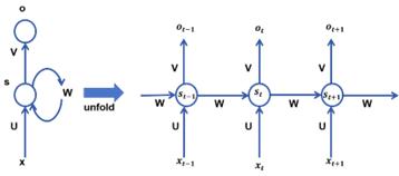
Figure 2. RNN network result diagram

Where \( x \) represents the input layer, \( o \) represents the output layer, \( s \) represents the hidden layer, and \( U \) , \( V \) , and \( W \) represent the weight parameters. At time \( t \) , the input of the hidden layer \( s_t\ \) contains, in addition to the output of the input layer at the current time, the output state of the hidden layer at the previous time \( s_{t - 1} \) .

The formula of forward propagation process in RNN is as follows:

\( o_t=g(V_{s_t}) \) (2)

\( s_t=f(U_{x_t}+W_{s_t - 1}) \) (3)

As can be seen from the above formula, RNN recurrent neural network has an extra weight matrix \( W \) added to the hidden layer compared with the traditional ordinary neural network. The hidden layer in every moment of RNN can complete the memory of the information of the previous moment, but in practice, there will be gradient disappearance or gradient explosion. Therefore, The hidden layer \( s_t \) in the RNN completes only the short-term memory of the information.

3.3. Long short term memory neural network prediction model

Long Short Term Memory (LSTM) [8] Unlike feedforward neural networks, LSTM can use time series to analyze the input. After the RNN prediction of carbon emissions, it is found that gradient disappearance occurs in the prediction process. Therefore, in order to avoid gradient disappearance, this paper uses the LSTM model to compare with the RNN model. Compared with the RNN neural network model, the conventional neurons of LSTM are replaced by storage units. The specific structure of a single LSTM neuron is shown in Figure 3 [9]:

Figure 3. Single LSTM neuron structure

\( F_t=\varphi(X_tW_{xf}+h_{t - 1}W_{hf}+b_f) \) (4)

\( I_t=\varphi(X_tW_{xi}+h_{t - 1}W_{hi}+b_i) \) (5)

\( {\widetilde{C}}_t=tanh{(}X_tW_{xc}+h_{t - 1}W_{hc}+b_c) \) (6)

Where \( X_t\ \ \) is the input sequence of the network structure at time \( t \) , \( h_{t - 1}\ \) is the output of the hidden layer at time \( t - 1 \) , and the above mentioned \( W \) and \( b \) are the weight parameters that need to be updated by the chain rule. Formula 4 is the forgetting gate, and formula 5 and 6 are the input gate. By combining formulas 4, 5 and 6, the state value of the cell at the current moment can be obtained namely \( C_t \) :

\( C_t=F(t)\otimes C_{t - 1}+I_t\otimes{\widetilde{C}}_t \) (7)

The value of the hidden layer \( h_t \) at the next time can be obtained by using the cell update value \( C_t \) , as follows:

\( o_t=\varphi(X_tW_{xo}+h_{t - 1}W_{ho}+b_o) \) (8)

\( h_t=o(t)\otimes t a n h{(}C_t) \) (9)

Formulas 8 and 9 represent output gates. The \( \varphi \) activation function involved above is a function of \( sigmod \) belonging to \( 0 - 1 \) , the forgetting gate is approximately equal to 1, the input gate is approximately equal to 0, and the output gate can be approximately equal to 0 or 1, depending on whether the information is passed.

3.4. Other machine learning algorithms

3.5. Extreme gradient lifting tree

The basic components of Extreme Gradient Boosting (XGBoost) [10] are decision trees, which have sequence among them. The generation of the latter decision tree depends on the prediction results of the previous decision tree, that is, the deviation of the previous decision tree is taken into account, so that the training samples with poor prediction of the previous decision tree receive more attention in the follow-up, and then the next decision tree is trained based on the adjusted sample distribution.

For XGBoost, although it can accurately find the data segmentation points, the algorithm needs to save not only the feature values of the data, but also the results of its feature ordering, resulting in a larger space required. Meanwhile, when traversing the segmentation points, XGBoost needs to calculate the information gain, which makes the time longer.

3.6. Lightweight gradient elevator

The Light Gradient Boosting Machine (LightGBM) [11] algorithm can well solve the shortcomings of XGBoost, and the algorithm idea is shown in Figure 4:

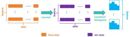
Figure 4. Histogram of LightGBM algorithm

Compared with XGBoost, the model does not need to store the pre-ordered results, but only needs to store the discretized values of the features. In addition, compared with XGBoost which needs to calculate the gain of one split when traversing an eigenvalue, LightGBM method only needs to calculate k times, which greatly improves the storage efficiency and reduces the operation time.

3.7. Random forest

Random forest [6]is an ensemble learning machine learning algorithm that makes regression predictions by building and combining multiple decision trees. The specific steps are shown in the figure 5:

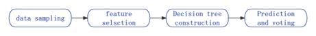
Figure 5. Steps of random forest algorithm

Compared with other algorithms, random forest algorithm has higher stability. Even if new data is added to the data set, it can only affect one decision tree and will not have a greater impact on the whole algorithm.

3.8. Stacking algorithm fusion

The ensemble algorithms boosting and bagging are combined in the Stacking algorithm [12], which uses multiple base learners to learn and hand the learned data to the second layer learner, the metmodel, for fitting and prediction. In the previous paper, three algorithms, XGBoost, LightGBM and Random forest, were used to fit and predict. In order to make the fitting effect more accurate, the three algorithms above were used as the base model and linear regression was used as the metametter to integrate the Stacking algorithms and again to fit and predict the carbon dioxide content in the Alps.

In order to prevent overfitting in the Stacking algorithm, the \( k \) -fold cross-check method is used in this paper. The principle is to divide raw data into \( k\ \ \) groups, one part of which is used as the training set and the other part as the verification set, and only \( k - 1 \) groups are trained for each training. Repeating the above process can prevent overfitting of the model.

3.9. Machine learning hyperparameter optimization

Since machine learning models need to be used many times in this paper, and model parameters need to be adjusted in machine learning, there are two mainstream methods for finding hyperparameters of models at present, network search and random search. However, in practice, it can be found that both of them have the disadvantage of consuming too much time, and when there is a large amount of data, the time consumed increases exponentially.

In order to solve the problems caused by the above two parameter optimization methods, this paper uses the Bayesian optimization algorithm[13], which is more efficient than other global optimization algorithms. Its principle is that after the objective function is given, the posterior distribution of the objective function is optimized by adding sampling points until the posterior distribution gets the optimal model hyperparameter combination.

4. Model solving and result analysis

4.1. Data selection and preprocessing

In order to accurately predict world Carbon dioxide emissions, this paper collected real-time 8,487 data on the Zugspitze mountain in the Alps from April 1, 2023 to May 1, 2024 based on the Integrated Carbon Observation System (ICOS). The scatter plot of carbon dioxide emissions from Zugspitze Mountain after data pretreatment is shown as follows:

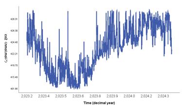
Figure 8. Preprocessing of carbon dioxide emission data in the Alps

4.2. Neural network prediction model

In this paper, parameters of RNN and LSTM are optimized based on Bayesian optimization algorithm. And mean square error( \( MSE=\frac{1}{n}\sum _{i=1}^{n}{(x_i} - {\hat{x}}_i)^2 \) )､the root mean square error( \( RMSE=\sqrt{\frac{1}{n}\sum _{i=1}^{n}{(x_i} - {\hat{x}}_i)^2} \) )and goodness-of-fit( \( R^2=1 - \frac{\sum _{i=1}^{n}{(x_i - {\hat{x}}_i)^2}}{\sum _{i=1}^{n}{(x_i - \mu)^2}} \) )three evaluation index were analyzed｡Where \( {\hat{x}}_i \) is the predicted value of \( x_i \) .Comparison and prediction results are shown in Figure 9-10 and Table 2:

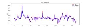
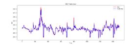
Figure 9. LSTM prediction results Figure 10. RNN prediction results

Table 2. Comparison of neural network prediction results

The results show: When the number of iterations is both 25, the \( MSE \) and \( RMSE \) of RNN are both higher than LSTM, and the goodness-of-fit \( R^2 \) is lower than LSTM, indicating that LSTM is superior to RNN under this condition. The influence of data volume on LSTM was further analyzed. In this paper, 8487 data were randomly selected, with sample sizes of 500, 1000 and 3000. Moreover, 25 iterations were performed respectively, and the results are shown in Figure 11-14 and Table 3:

Table 3. Comparison of prediction results with different sample sizes

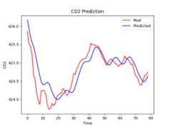
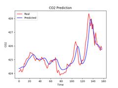
Figure 11. Sample size is 500 Figure 12. Sample size is 1000

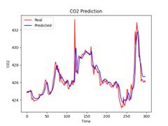
Figure 13. Sample size is 3000 Figure 14. Sample size is 8487

It can be seen from Table 3 that with the increase of data volume, the fitting effect of LSTM shows an upward trend. When the data volume reaches 8487, the goodness-of-fit \( R^2 \) of LSTM can reach 0.89. Therefore, the LSTM prediction model is suitable for big data analysis.

In order to detect the influence of iterations on LSTM, all data were used in this paper and prediction experiments were conducted based on iterations of 10, 25, 50 and 100 respectively. The results are shown in Figure 15-18 and Table 4:

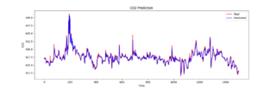
Figure 15. Iterates 10 times Figure 16. Iterates 25 times

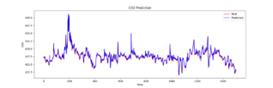
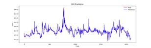
Figure 17. Iterates 50 times Figure 18. Iterates 100 times

Table 4. Comparison of prediction results of different iterations

According to Table 4, as the number of iterations increases, the goodness-of-fit \( R^2 \) gradually rises to close to 1, while \( MSE \) and \( RMSE \) show a downward trend.

In order to accurately predict the carbon dioxide content in the Alps, this paper selected the carbon monoxide content and methane content in the Alps as factors affecting the carbon dioxide content in the air[14]. The results are shown in Figure 19-22 and Table 5:

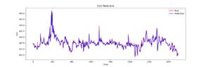
Figure 19. CO2 (LSTM) Figure 20. CH4-CO2

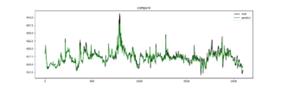
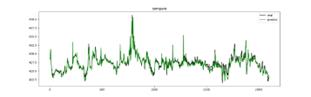
Figure 21. CO-CO2 Figure 22. CO-CH4-CO2

Table 5. Comparison of prediction results of different influencing factors

It can be seen that when both carbon monoxide and methane are added to the model, the prediction effect is better, the goodness-of-fit \( R^2 \) can reach 0.95, and the \( MSE \) is only 0.22. Therefore, when more influential factors are added to the LSTM prediction model, the fitting effect will be better.

4.3. Other machine learning and Stacking prediction models

In order to reduce the running time of the prediction model, this paper replaces the LSTM neural network model with other machine learning models, such as XGBoost, LightGBM, and Random Forest prediction model[15]. The parameters of the three algorithms were optimized according to Bayesian optimization algorithm, and the corresponding prediction results were obtained, as shown in Table 6:

Table 6. Comparison of other machine learning predictions

In order to improve the fitting effect of three models, the paper uses the fusion method of Stacking algorithms to essentially aggregate the advantages of three machine learning models. The final prediction results are shown in Figure 23:

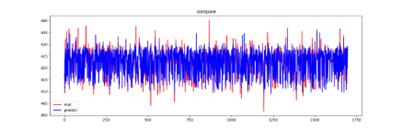
Figure 23. Prediction results of Stacking

It can be seen from Table 6 that three reference indicators of the Stacking model are superior to three base models. Therefore, the fusion of Stacking algorithms has higher fitting degree and better fitting effect than three base models.

5. Sensitivity analysis

Sensitivity test is a test method to study the sensitivity of a model's state and output changes to system parameters. Sensitivity analysis is often used in algorithms such as machine learning to study the stability of parameters when they change. Sensitivity analysis can also be used to see which parameters have a critical impact on the model. Therefore, in order to ensure the stability of the experimental results, this paper will analyze the results of the prediction model through the sensitivity test. Because there are many models in this paper and the parameters are relatively complex, the number of trees in the random forest is used as the parameter variable and the Stacking model is used to predict. The results are shown in Figure 24:

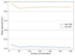
Figure 24. Sensitivity test

It can be seen from the figure that when parameters (the number of trees) change, the prediction fitting results of the Stacking model do not change significantly. Therefore, the model has high stability.

6. Conclusion

With the large amount of greenhouse gases, including carbon dioxide, discharged, the world temperature has risen across the board, and people's lives have been seriously affected, so accurate prediction of carbon dioxide content has become crucial. In this paper, RNN and LSTM neural network models are used to predict the carbon dioxide content in the air over the European Alps, respectively. The results show that the fitting effect of LSTM is better than that of RNN, and the fitting effect will increase with the increase of sample size or number of iterations. At the same time, the content of methane and carbon monoxide in air was added to the LSTM as a prediction model of influencing factors, and the experimental results showed that the determination coefficient \( R^2 \) could reach 0.95, which was higher than the prediction results with single influencing factors or no influencing factors. In order to reduce the running time, this paper uses XGBoost, LightGBM, and random forest as the base models and linear regression as the meta-model to perform prediction experiments. The determination coefficient \( R^2 \) can reach 0.92. Finally, the sensitivity analysis of the Stacking fusion model is carried out in this paper. The experimental results show that the model has strong stability.

References

[1]. Sharif Hossain M. Panel. “stimation for CO2 emissions, energy consumption, economic growth, trade openness and urbanization of newly industrialized countries,” Energy Policy(2011):6991-6999.
[2]. C Zhang, Y Lin. “Panel estimation for urbanization, energy consumption and CO2 emissions: A regional analysis in China,” Energy Policy(2012):488-498.
[3]. Q Y Lu, Y Zhang, S S Meng, et al. “A review of carbon peaking prediction methods under the "two-carbon" target ,” Journal of Nanjing Institute of Technology (Natural Science Edition)(2022): 68-74.
[4]. Haijie Wu, Lianzhi Wang, Min Xie, et al. “Prediction of electric power carbon emission peak based on grey BP neural network,” Electronic Design Engineering(2024): 105-109.
[5]. Lili Zhang, Mingdong Tang. “Prediction of road carbon emission concentration based on recurrent neural network model,” Transportation Science and Economics(2024): 23-30.
[6]. Swetha P S,Sshakthi M A C, et al. “Prediction of column average carbon dioxide emission using random forest regression,”Proceedings of Data Analytics and Management. Singapore: Springer Nature Singapore(2024): 377-388.
[7]. Mainoc, Misul D, Di Mauro A, et al. “A deep neural network based model for the prediction of hybrid electric vehicles carbon dioxide emissions,” Energy and AI(2021).
[8]. J Meng, G Ding, L Liu. “Research on a prediction method for carbon dioxide concentration based on an optimized lstm network of spatio-temporal data fusion,” IEICE Transactions on Information and Systems, E104D(10)(2021): 1753 - 1757.
[9]. C Wang, F Xie, J Yan, et al. “A u-midas modeling framework for predicting carbon dioxide emissions based on lstm network and lasso regression,” SSRN(2024).
[10]. Chenguang Wang, et al. “Permafrost strength prediction and influencing factors analysis based on XGBoost algorithm,”(Metal mines): 1-14.
[11]. Jieru Gao, Linjing Wei, et al. “Prediction model of PM2.5 concentration based on Prophet-LightGBM,”Software Guide:1-9.
[12]. Liang Z H, Ying Z Q, Liu M M, et al. “Prediction Method of rust expansion and Crack of Reinforced Concrete Based on the Integration of Stacking Model ,”Chinese Journal of Corrosion and Protection: 1-13.
[13]. Q Song, Y L Bay, R Wang, et al. “Ensemble framework for multistep carbon emission prediction: An improved bi-lstm model based on the bayesian optimization algorithm and two-stage decomposition,” SSRN(2024).
[14]. Y X Huang. “Analysis of influencing factors and prediction of industrial carbon emission in Shanghai,” Shanghai University of Finance and Economics(2023).
[15]. Yihan Liu. “Analysis of Key Influencing Factors of low-carbon development of freight transport and Prediction of carbon emission reduction,” Beijing Jiaotong University(2023).
Cite this article
Wu,Y.;Duan,Q.;Sui,J. (2024). Prediction of carbon dioxide levels in the European Alps based on machine learning algorithms. Applied and Computational Engineering,95,23-33.
Data availability
The datasets used and/or analyzed during the current study will be available from the authors upon reasonable request.
Disclaimer/Publisher's Note
The statements, opinions and data contained in all publications are solely those of the individual author(s) and contributor(s) and not of EWA Publishing and/or the editor(s). EWA Publishing and/or the editor(s) disclaim responsibility for any injury to people or property resulting from any ideas, methods, instructions or products referred to in the content.
About volume
Volume title: Proceedings of the 6th International Conference on Computing and Data Science
© 2024 by the author(s). Licensee EWA Publishing, Oxford, UK. This article is an open access article distributed under the terms and
conditions of the Creative Commons Attribution (CC BY) license. Authors who
publish this series agree to the following terms:
1. Authors retain copyright and grant the series right of first publication with the work simultaneously licensed under a Creative Commons
Attribution License that allows others to share the work with an acknowledgment of the work's authorship and initial publication in this
series.
2. Authors are able to enter into separate, additional contractual arrangements for the non-exclusive distribution of the series's published
version of the work (e.g., post it to an institutional repository or publish it in a book), with an acknowledgment of its initial
publication in this series.
3. Authors are permitted and encouraged to post their work online (e.g., in institutional repositories or on their website) prior to and
during the submission process, as it can lead to productive exchanges, as well as earlier and greater citation of published work (See
Open access policy for details).