


1. Introduction
Power systems become one of the most critical infrastructures, supplying a steady source of electricity to millions of consumers around the country and becoming the backbone of rapid urbanization in Asia regions. Modern power systems need to be prepared to survive low-frequency impact events such as natural catastrophes (2020 Bengal), extreme weather conditions (2021, China), pandemics (Covid-19), etc., to guarantee the full functioning of an electricity-dependent society.
Reducing the restoration time of a failed power system is critical for enhancing system resilience effectively and efficiently. During the restoration process, the power system is not just an isolated system but coupled with other critical infrastructures such as the water supply station and hospitals. The interdependency is ignored during the restoration process it can lead to inaccurate disaster assessment (cascading failure analysis), uncoordinated recovery, and a long decision-making period, ultimately resulting in low system resilience against disasters. Resilient power systems are crucial for developing Asian countries, where economic growth depends on an uninterrupted electricity supply. It is estimated that China loses about 1.44 billion yuan in the business sector during an outage event [1]. The shortening of the restoration time and the investigation of interdependencies between the critical infrastructures has become a top priority to effectively and efficiently minimize the losses.
Resilience needs to be integrated into planning and operational assessment to design and operate adequately resilient power systems considering the interdependencies between the Power system and the other critical infrastructure. To evaluate the performance of a single network is insufficient thus a new resilience is defined for a coupled network, for example, reliability is widely used for evaluating the delivered quality of service for a single power system.
2. Literature Review
Recent efforts have been researching the power system’s resilience optimization against disasters. The restoration optimization problem is modeled as a complex non-convex optimization in [2]. The application of mixed-integer linear programming in this problem facilitates independent decision-making within subsystems. To enhance restoration solutions in specific conditions, [3] aims to develop a power system restoration model for power transmission systems that can adjust restoration solutions in specific blackout scenarios or weather conditions. A reformulated model is proposed to relieve the burden of complex power system restoration problems. While [4] proposes a bi-level coordinated power system restoration model that also considers the support of multiple flexible resources, for instance, the batteries. This study integrates three stages: black-start zone partitioning, network reconfiguration, and load restoration. In the existing research, collaborative recovery of critical systems is not taken into consideration. As discussed above, the power system’s resilience can be improved by taking the interdependency of the network and critical infrastructure into account.
[5] uses a deep Q-network to optimize load-shedding (DQN-LS) strategy and maintain power system stability in an operating power system. The DQN-LS can provide accurate and real-time decisions to increase the quality and probability of voltage recovery during a power system fault. Emergency load shedding is commonly used to prevent continuous frequency drops and power outages. To more effectively deal with an outage, [6] proposes a data-driven load-shedding strategy, which incorporates deep Q learning. This strategy can obtain the load-shedding decision that best maintains a stable power supply for important loads and reduces decision-making time.
In addition to the manual recovery to enhance the resilience of a distribution system after a major outage, [7] proposes Reinforcement Learning to facilitate the automatic recovery process. This model acts as a robust decision-making tool for scenario analysis with asynchronous and partial information outages. Due to the uncertainty of the initial power system restoration, [8] develops an online generator start-up algorithm based on Monte Carlo tree search and sparse autoencoder. This algorithm can search for the next line to be restored with real-time decision-making capability. In [9], a microgrid formation restoration method using deep reinforcement learning is proposed. This method can reduce the length and impact of power outages, maintain continuous services, and improve reliability during outages. Furthermore, the application of machine learning algorithms, specifically regression techniques, in resilience optimization is rare in current research.
The major contributions of this research are outlined:
● Operational Interdependence Simulator (OIS) is proposed to simulate the interdependencies between critical infrastructures to help prioritize sequenced failure recovery based on the Operational Capacity Table (OCT).
● Critical Infrastructure Utility (CIU), a unified performance indicator, is defined to evaluate the restoration effectiveness, which is the reference to the proposed recovery algorithm.
● To eliminate all the time-consuming calculations (e.g., power flow calculation, system state evaluation, etc.), an AI agent is innovatively introduced, enabling fast online response for decision-making support during large emergency events.
The rest of this article is organized as follows. The system flowchart is introduced in Section II. The CIU is defined in Section III along with the OCT and interdependencies modeling. In Section IV, a detailed description of the restoration optimization including an AI agent and the optimal queue search is proposed. The results of the restoration optimization and algorithms are analyzed and discussed in Section V, followed by the conclusion in Section VI.
3. Problem Formulation (System Flowchart)
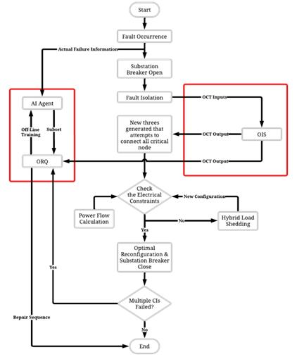
Figure 1. The overall flowchart of the proposed resilience enhancement strategy
Figure 1 illustrates the step-by-step process of the power system recovery with the red box highlighting the contributions of this research. For example, the restoration process is shortened and simplified through the AI agent and proposed OIS to simulate the interdependencies between critical infrastructures. In the event of a failure within the power system, the circuit breaker within the power system triggers an automatic opening to prevent further cascading damage to the rest of the system. Simultaneously, the system reports the number of faulty buses/branches and their respective locations, recording this information to the database for further analysis. The redundant lines then come into play, ensuring connectivity to the most important buses that connect the critical infrastructures. The determination of the optimal order of isolation is facilitated by OIS.
The Minimum Spanning Tree (MST) or Shortest Path Tree (SPT) Search algorithm is employed to generate a new topological reconfiguration that establishes the connections to critical nodes. Although all critical nodes are prioritized (compared to the non-essential ones), not all may be connected due to physical topology or electrical constraints. In cases where electrical constraints are violated, a load-shedding scheme is proposed that removes buses to alleviate the load and safeguard critical nodes. Alternatively, if no constraints are breached, an optimal reconfiguration and substation breaker close is recommended. The breaker is reclosed prior to operating the relative tie switches automatically.
After automation, the manual execution of the proposed Optimal Repair Queuing (ORQ) algorithm based on CIU values calculated from the OCT table is followed, aiming to rectify all faults and restore the power system to its initial state. To provide real-time decision support, the off-line trained AI agent suggests optimization restoration procedures directly and skips all the conventional checks.
Through these comprehensive steps, the system ensures a systematic and efficient recovery process in the face of power system failures.
4. The Resilience Assessment Approach
4.1. Resilience definition
Resilience is defined with the concept of N-1 to N-k, where k represents a number greater than one. This approach recognizes that multiple simultaneous failures (up to n) can occur and seeks to design methods that can adapt and recover from such multiple failures.
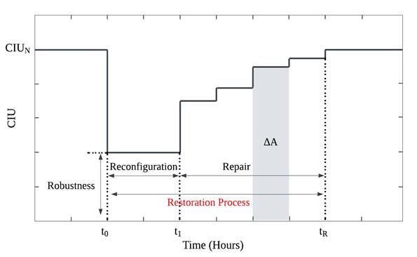
Figure 2. The illustrative curve that represents the proposed resilience quantification
Symbols |
Definition |
t0 |
The power system experiences failures, initiating the restoration process. The location of failures is sent for the calculation of a new reconfiguration. |
t1 |
The calculation of a new reconfiguration concludes, and the repair process begins. |
tR |
Upon completion of the repair, the power system reverts to its initial CIU value. |
CIUN |
The normal CIU value is when no failures are present in the power system. |
∆t |
Intervals during which the repair process occurs, resulting in a new CIU value at the end of each interval. |
The hours before \( t_o\ \) are the pre-event stage, where the power system is still fully operational and no failures (at least no major failures) have occurred.
The event/disaster occurs at t0, and the restoration process spans between \( t_o\ \) to \( t_R\ \) but is split into two sections.
From \( t_o\ \) to \( t_1\ \) , the proposed topological reconfiguration is executed, which will suggest a new reconfiguration of the power system, considering the reconnection of critical infrastructures.
The repair process begins at t1 and increases the CIU value of the coupled system by delta A at each repair action between \( t_o\ \) to \( t_R\ \) .
5) After the repair, the power system will return to its initial state with a CIU value back to 100% (CIU = CIUN when the entire city is fully functioning/under normal conditions).
\[ objective\ maximize\ R\ =\frac{\sum _{t_{0}}^{t_{R}} ∆t ∗ CIU(t)}{(t_{R} - t_{0}) ∗ 100%} \] (1)
The equation proposed aims to quantify the resilience of the system by accumulating the area under the curve from \( t_0 \) to \( t_R \) by multiplying the ∆t and the CIU(t) at that interval. This is divided by the total area of the same interval when CIU remains at 100%. The ratio yields a percentage from 0 to 100%, indicative of the speed of the system's resilience. The objective is to increase the percentage by emphasizing maximizing the area under the curve of the interval.
Assessing the performance of individual networks alone is insufficient, highlighting the need to create a new resilience framework specifically tailored for coupled networks. There are some inter-use of reliability, robustness, and resilience for the assessment of the new coupled network. While reliability focuses on the consistency of the performance of a single system under operational disruptions.
Reliability is defined via the N-1 standard which ensures that the power system is designed to tolerate the failure of any single component without causing a complete system failure. The extra redundancy helps maintain the continuity of the power supply and reduces the likelihood of interruptions, thereby defining the system’s level of reliability.
There are some common ways to measure reliability in power systems. For example, the System Average Interruption Frequency Index (SAIFI) measures the average number of sustained interruptions experienced by customers in a given period with sustained interruptions defined as any disruption lasting more than five minutes by IEEE. SAIFI can be improved by reducing the frequency of outages through better preventative maintenance. Improved equipment maintenance and tree trimming, for example, can limit the number of service interruptions.
\( SAIFI\ =\ \frac{Total\ Number\ of\ Sustained\ Interruptions}{Total\ Number\ of\ Customers\ Served} \) (2)
System Average Interruption Duration Index (SAIDI) measures the average duration of interruptions experienced by customers in a given period. SAIDI describes the total duration of the average customer interruption. Customer Average Interruption Duration Index (CAIDI) measures the average time it takes to restore power to customers after an interruption. Both of which can be improved by a quicker response to outages (a period when a power supply or other service is not available) is one of the most direct ways to improve SAIDI.
\( SAIDI\ =\ \frac{Total\ Duration\ of\ Sustained\ Interruptions}{Total\ Number\ of\ Customers\ Served} \) (3)
\( CAIDI\ =\ \frac{Total\ Duration\ of\ Sustained\ Interruptions}{Total\ Number\ of\ Sustained\ Interruptions} \) (4)
Robustness is a scenario-independent factor that needs to remain stable and perform efficiently in the presence of uncertainties in the system and its environment [10]. It is often embedded in the operation of the power system. Robustness is examined by considering how much performance (CIU) the coupled system can maintain during the event’s occurrence (“ \( t_o\ \) ” as shown in Figure 2). This does not involve the restoration and recovery portions after the disaster. However, the definition of resilience considers the system performance changes throughout the entire event(not only pre-disaster but also post-disaster). In addition, a resilience analysis will reveal strong couplings with other infrastructural systems (communications, water, transportation, etc.).
4.2. Operational Capacity Table (OCT)
Table 1. OCT that quantifies each infrastructure’s operational capacity
Output |
Inputs |
||||
Critical Infrastructure Utility |
Power supply (kWh per household per day) |
Water station (Liter per capita per day) |
Hospital (Percentage in operation) |
Government (Percentage in operation) |
ICT Executor (kbit/s) |
100% |
40 |
140 |
100% |
100% |
260 |
75% |
30 [11] |
100 [13] |
80% |
75% |
190 [12] |
50% |
20 |
60 |
60% |
50% |
120 |
25% |
10 |
20 |
30% |
25% |
60 |
0% |
0 |
0 |
0 |
0 |
0 |
*According to [11], the power supply for a household is 30 kWh per day, and 190 kbit/s usage is stated by [12]. The average water consumption for a small city is 100 liters per capita per day according to [13].
Table 1 is an example of OCT, the inputs are crucial factors for the functioning of the city/community (for example, the water supply). OCT is used to quantify the operational capacity of each infrastructure component and understand the interdependencies between various factors. It guides the prioritization and allocation of resources for each input for sequenced failure recovery. The OCT ensures that restoration efforts consider the interdependencies, preventing isolated efforts that may not contribute to overall system recovery. In the example shown in Table I, the lowest highlighted section is the water station. Thus, there will be a prioritization of water stations, and when the limiting resources are increased, it would improve the CIU value.
The output (CIU) represents the percentage of operational critical infrastructure. The inputs are crucial factors for the functioning of the city/community. OCT provides guidance on the priority and allocation of resources for each recovery action considering their interdependencies.
The output column (left column) of Table I is the CIU and the input columns are the power supply in kWh per household per day, the hospital’s medical service output in percentage in operation, ICT Executor in kbit/s, the government facility, along with water station in Liter per capita per day. The initial relationships are established in the form of nonlinear rational function and there is a unique relationship between individual input and the output (for example, power supply per household and CIU in Table I). It often involves the use of surveys, questionnaires, and qualitative assessments to capture occupants' preferences and perceptions (to characterize the relationship). Yellow is used to highlight the section of the box that is the minimum performance level input at a certain CIU output. If one of the inputs is on the defined bottom line, then regardless of how high the performance level of the other inputs is, the output, CIU, does not increase. This allows the operator to easily identify the input that is limiting the output, so they can allocate resources to the input efficiently. CIU indicates the level of recovery in the system, which is the reference (input data) for the offline training.
The overall purpose of proposing OCT is to provide a more user-friendly approach to knowing the limiting resource of each critical infrastructure and the cascading mechanism between the CIs during a failure. The inputs and outputs are also converted into a finite number which not only eases the reading but also simplifies the calculation and sensitivity to change. For example, it is more readable if the operators can visualize the inputs as a value such as 25%, 100%, etc. rather than in mathematical formulas. Since all of the inputs are not in the same category (with identical units) thus it would be illogical to simply add the values, the table gives a unified CIU value, linking the individual relationship between the input and the output. Additionally, the readability of the table will help guide an operator in the restoration procedures, increasing the overall resilience of critical infrastructure by efficiently managing recovery resources.
4.3. Operational Interdependence Simulator (OIS)
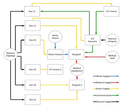
Figure 3. An illustrative example of the OIS
In Figure 3, circles are used within the diagram to define the sources in the system that only provide output supply to other points and don’t have any input and rectangles that stand for the critical infrastructures that have inputs from other dependent CIs or resources. To help the operators identify the different supplies that are being provided to different critical infrastructures, color is used to label each. For example, the “red” line is the medical supply that provides the resources needed for the hospital, allowing it to function, and the “yellow” line is the power supply that provides the electricity that many critical infrastructures need, etc, creating a basic model of the. Overall, the OIS is implemented in this research to better visualize the interdependence between each infrastructure in a system and to calculate the CIU changes induced by interdependencies for each simulation.
5. Restoration Optimization
5.1. Optimal Repair Queuing (ORQ) Algorithm
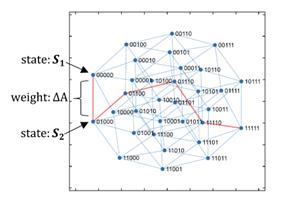
Figure 4. The graphical representation of ORQ strategy
If there are critical components/nodes that can’t be reconnected via reconfiguration physically, a manual repair must take place. However, due to the limited resources, it is difficult to repair everything at once thus an optimal order needs to be proposed to optimize with considering resilience maximization. Figure 4 shows the optimal queue for recovery (an illustrative use case) based on a queue search algorithm, which determines the optimal path for recovery.
At each state (for example Sate 1: S1 or Sata 2: S2 in Figure 4), the OIS outputs the CIU value to determine the weight between each transient. ∆A in Figure 2 stands for the amount of recovered system performance based on CIU multiplied by the time it takes to repair one component. ∆A is calculated as ∆t times CIU(t) and is equal to the weight in ORQ.
The red path corresponds to the optimal restoration queue for faulted feeders which are determined by the proposed method. The number of faults or feeders is shown by the number of digits with damaged ones labeled as 0 and 1 as repaired/normal. In this example, the optimal restoration queue is feeder 2, feeder 3, feeder 4, feeder 1, and finally feeder 5. The repair process ends with all of the digits displayed with 1s. The ∆A can be converted to weight by multiplying negative 1 thus converting ∆A from maximization to minimization.
5.2. Graph Theory and Adjacency Matrix
Graph Theory is the study of the relationship between the vertices (nodes) and edges (lines). A tree in a graph is the connection between undirected networks which have only one path between any two vertices. A “degree” in a graph is mentioned to be the number of edges connected to a vertex. A “cycle” in Graph Theory is a closed path in a graph that forms a loop. If there are n vertices in the graph, then each spanning tree has \( n - 1 \) edges.
Adjacency Matrix (also called the connection matrix), an important concept in Graph Theory, is applied in this research to represent the power network so that the computer can understand the topology of the network and implement the reconfiguration algorithms. It is a matrix containing rows and columns that are used to represent a simple labeled graph, with 0 or 1 in the position of (Vi, Vj) according to the condition of whether Vi and Vj are adjacent or not. If there is an edge between vertex i and vertex j, A[i, j] is typically set to 1 or may contain a weight value if the graph is weighted. If there is no edge between vertex i and vertex j, A[i, j] is typically set to 0.
5.3. Minimum Spanning Tree and Shortest Path Tree
Restoring electrical service is a crucial aspect of power system restoration, and MST and SPT are employed in this process. The MST’s primary objective is to connect all the nodes, without any cycles, and with the minimum possible total edge weight. MST offers an approach that prioritizes the selection of lines based on resource availability and economic viability, ensuring the efficient restoration of electrical service.
On the other hand, SPT addresses a different facet of power system restoration. Their primary objective is to establish the shortest and most efficient electrical paths from substations, which optimize power flow and minimize transmission losses. During power system restoration, SPT allows operators to identify the shortest paths from the root node to crucial loads to reestablish power delivery. In both algorithms, nodes can be disconnected if they are situated in an unreachable position (this violates the operational constraints).
5.4. Load shedding
In power distribution systems, before reclosing the circuit breaker, the operator should make sure the new topological configuration meets the basic electrical constraints. If a bus is far away from the substations, especially when the bus is not fed by a usual substation, it may suffer a significant voltage drop. The longer the distance, the greater the resistance in the lines, leading to a more significant voltage drop. Network topology determines how loads are distributed and connected, which can alleviate voltage level-related issues. Network topology can also influence the performance of voltage regulation, the process of maintaining voltage levels. Load shedding is used to eliminate voltage collapse risk during power delivery, which is usually designed for critical points to compensate for voltage drops. The method will remove (based on the electrical constraints, (5), (6)) the non-critical nodes to protect critical nodes.
\( V_i^{min}\text{<}V_i\text{<}V_i^{max},i \in I\ \) (5)
\( \left|I_f^{min}\right|\text{<}\left|I_f\right|\text{<}\left|I_f^{max}\right|,f \in F\ \) (6)
Equations (5) and (6) are used to determine the topological reconfiguration. \( V_i \) is the voltage at the node \( i \) with \( I_l \) representing the current at the current feeder \( f \) . These values are bounded between the voltage min and max, and the current min and max respectively.
5.5. AI Agent
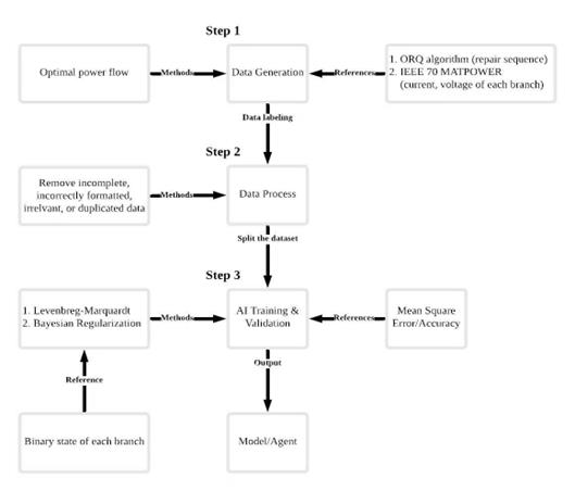
Figure 5. The flowchart for the training of the AI agent
AI is implemented due to the complexity of decision-making in the restoration process of critical infrastructures. Offline training allows AI to bypass the complicated decision-making processes, enabling it to propose the optimal restoration route in real time and reducing computation time.
Step 1: The ORQ algorithm is implemented by checking the CIU values calculated from the OCT table, whose results serve as the output of the AI agent training. IEEE 70 MATPOWER is used to generate the offline data. IEEE 70-bus system parameters are loaded and optimal power flow calculations based on Newton Raphson equations are used to calculate the power flow, yielding a new dataset (system states).
Step 2: Data collection in this research includes power system data acquisition (i.e., current, and voltage of each branch via MATPOWER), data labeling (restoration sequence with the corresponding resilience index), and existing data/models pre-processing. The implementation also involves removing incomplete, incorrectly formatted, irrelevant, or duplicated power data and recovery decisions. Once processed, the dataset is split into three groups for the following training, validation, and testing procedures with a recommended ratio of 70/15/15 or 80/10/10, respectively.
Step 3: Levenberg-Marquardt (LM) algorithm and the Bayesian Regularization (BR) are used algorithms as a training method in the AI model. The LM algorithm starts by guessing the parameters of the mathematical model. It then iteratively adjusts these parameters to minimize the sum of squared residuals to fit the observed data. This approach ensures a more stable and convergent optimization process. The BR algorithm is an alternative training method in the AI model. First, the relevant features of the data used for classification are identified. Based on Bayes' theorem and the naive independence assumption, the algorithm selects the class with the largest posterior probability by calculating the conditional probability of the observed data under each class.
The binary states of each branch are used as the inputs of the BR/LM algorithm with Linear regression used to validate the training. In general for validation, the closer the data points are to the regression line, the more accurate the final output (the decisions of which part to recover first) is. Higher deviations between data points and the regression line (45-degree line) result in less precise predictions. The correlation coefficient, denoted “r”, is a unit-free value between -1 and 1 that quantifies the linear relationship. P-value is used to evaluate statistical hypothesis testing results. A P-value less than the significance level (usually 0.05) is considered statistically significant, while a P-value greater than 0.05 indicates there is no significant linear relationship between the input variable(s) and the output. Mean Square Error (MSE) is also calculated by taking the square of the difference between all observed values and the predicted value. The sum of those squared values and divided by the number of observations. Accuracy is a metric used in this research that measures how often a machine learning model correctly predicts outcomes; however, too high of accuracy may not be optimal as it can lead to underfitting and overfitting, where the model performs too accurately only on training data or performs poorly on both datasets, resulting in worse decisions.
6. Tests and analysis
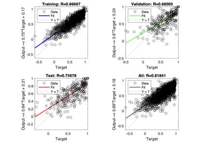
Figure 6. Regression results of system resilience by LM
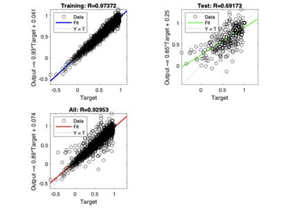
Figure 7. Regression results of system resilience by BR
Figure 6 and Figure 7 show the relationship between the network outputs and the targets with 10 hidden layers used. If the training was perfect, the output and the targets would be equal, as indicated by the dashed line, but that rarely occurs. Each data point is shown in the graph, and a solid line is used to represent the best-fit linear regression line between the actual outputs and the targets. Note that the ORQ can also be attached in the output for each scenario during the training process, ensuring that the agent understands and yields both resilience and ORQ results online.
Datasets are split into three groups with the validation data used to measure network generalization and to stop training when generalization stops improving, which is seen in Figure 7. The test does not affect the network formation, thereby providing an independent measure of network performance during and after training.
The BR algorithm does not require a validation data set because BR has its form of validation built into the algorithm. The algorithm checks the model's performance based on how large the weights are. The larger the weights, the higher the error. This means that at the training stage if the validation step is on, it may not ever let the network explore larger weights, even though larger weights may lead to the global minimum. This explains why only three charts are displayed in Figure 6 while there are four in Figure 7.
With the same data set, the BR has a much higher R-value (0.97372) than LM’s R-value (0.86667), suggesting a better performance and accuracy on the training data set. Despite the better performance in training, BR failed to evaluate the relationship between the outputs and the targets, having an R-value of 0.69173 much lower than LM’s R-value of 0.73678. The discrepancy between the training and test performance suggests a potential issue with overfitting in the BR model. Overfitting occurs when a model learns the training data too well, capturing noise and specific patterns that may not generalize well to new, unseen data.
The number of hidden layers and neurons per layer greatly influences the complexity of the model. More hidden layers can potentially capture complex patterns in the data, but they also increase the risk of overfitting. On the other hand, having too few hidden layers or neurons may result in underfitting, where the model fails to capture important patterns in the data.
The LM algorithm is designed to find a local optimum. As an optimization algorithm, the LM may find a minimum that is a good solution within a specific region but not the overall best solution for the entire problem, converging to a local optimum rather than a global one. Compared to the LM algorithm, AI-assisted decision-making in disaster response using the BR algorithm has better global optimization because it considers more data points initially thus ensuring that it can find the absolute minimum and not a local minimum.
There is a trade-off between accuracy and simplicity. This is often referred to as the "accuracy-complexity trade-off." Achieving a high level of accuracy in a model may require increased complexity, which can make it take more time to compile. The LM algorithm usually requires less time. The training stops automatically when the generalization stops improving. However, the BR algorithm usually requires more time but may result in better generalization for data sets. The training finishes according to the adaptive weight minimization [14].
Table 2. Comparison between two training algorithms using 10 and 20 hidden layers
| Algorithms | Metric | Train 10 | Train 20 | Vali 10 | Vali 20 | Test 10 | Test 20 | All 10 | All 20 |
| Bayesian Regularization | MSE | 0.0042 | 0 | NaN | NaN | 0.0505 | 0.0819 | NaN | NaN |
| R | 0.9737 | 1.0000 | NaN | NaN | 0.6917 | 0.5864 | 0.92953 | 0.91728 | |
| Levenberg- Marquardt | MSE | 0.0205 | 0.0181 | 0.0458 | 0.0486 | 0.0386 | 0.0461 | NaN | NaN |
| R | 0.8667 | 0.8843 | 0.6801 | 0.6806 | 0.7368 | 0.6849 | 0.81841 | 0.82384 |
Table 2 shows the results of the training. The columns in the table show the MSE and R values of the training, validation, and test phases for both algorithms' hidden layers of 10 and 20. Validation 10 and 20 are not displayed in the BR algorithm column as it does not require a validation data set. 10 hidden layers are chosen as the 20 hidden layers display an occurrence of overfitting, leading to inaccurate results in the test data set. The BR algorithm has a significantly better MSE and R in the training data, however, a worse performance with new and unseen data sets in testing.
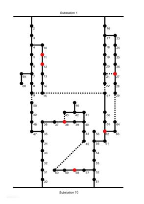
Figure 8. The topology of the IEEE-70 node power system with tie switches and critical nodes highlighted
Figure 8 shows the configuration of the power system used for the test that produces the results displayed in Table II. The interrelationships between each node are displayed with the critical nodes in red. The two substations 1 and 70 are at both ends, providing power to ensure the functionality of the system. The dotted lines are the redundant lines that provide alternative pathways for electricity to flow, during a failure, ensuring the critical nodes that are connected to the substation and are in operation.
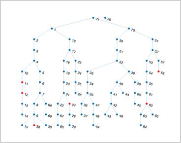
Figure 9. Topological reconfiguration using Shortest-Path Tree
Figure 9 is a topological reconfiguration result using the Shortest-Path Tree when 20 faults are applied on random branches. Each node is represented in Figure 9 with the red ones signaling critical infrastructures that are the most important ones that need to be recovered. 56 is disconnected from the rest of the topology because, as seen in Figure 9, the line between 55 to 56 has a failure, and there is no alternative line that will reconnect 56, resulting in a position that is isolated and physically unable to be reconnected. The purpose of the algorithm is to prioritize the recovery of the critical infrastructures by placing them closer to the source node or substations 1 and 70 to ensure that the important infrastructure load is not removed during load shedding.
Table 3 below compares the total computational time with and without using AI agents. Normally the decision response has to wait for all the solutions before obtaining a final answer, including the time needed for the simulation time of OIS electrical constraints check, topological reconfigurations, etc., to find the ORQ, (the conventional path that excludes the lighted AI part). With the AI agent's assistance, the solution step jumps from “Fault Occurrence” directly to the AI agent and then to the “ORQ”. This makes a huge time saving for the entire decision-making process.
Table 3. Comparison of the Computational Time with and without AI-assisted
Scenario |
Total time |
Base Solution |
2.6 hours |
AI embedded Solution |
7.3 seconds |
7. Conclusion
This research aims to enhance the resilience of critical infrastructures and the coupled power network. An OCT that quantifies each infrastructure’s operational capacity is proposed, along with the OIS to help prioritize the queue of failure recovery. The information is passed to the CIU which assesses restoration effectiveness and serves as a reference for the proposed ORQ algorithm. To accelerate the decision-making process, AI agents are introduced, resulting in more efficient artificial intelligence for disaster response. Reducing the restoration time of a failed power system is critical to effectively and efficiently enhance system resilience and help a city’s recovery. The proposed model can be applied to a multitude of fields such as emergency command, disaster services, post-disaster recovery, etc.
References
[1]. Chen, H., Yan, H., Gong, K., Geng, H., & Yuan, X. C. (2022). Assessing the business interruption costs from power outages in China. Energy Economics, 105, 105757.
[2]. Zhao, J., Wang, H., Hou, Y., Wu, Q., Hatziargyriou, N. D., Zhang, W., & Liu, Y. (2020). Robust distributed coordination of parallel restored subsystems in wind power penetrated transmission systems. IEEE Transactions on Power Systems, 35(4), 3213-3223.
[3]. W. Liu, J. Zhan, C. Y. Chung and L. Sun, "Availability Assessment Based Case-Sensitive Power System Restoration Strategy," in IEEE Transactions on Power Systems, vol. 35, no. 2, pp. 1432-1445, March 2020.
[4]. Liu, S., Chen, C., Jiang, Y., Lin, Z., Wang, H., Waseem, M., & Wen, F. (2022). Bi-level coordinated power system restoration model considering the support of multiple flexible resources. IEEE Transactions on Power Systems, 38(2), 1583-1595.
[5]. J. Zhang, Y. Luo, B. Wang, C. Lu, J. Si and J. Song, "Deep Reinforcement Learning for Load Shedding Against Short-Term Voltage Instability in Large Power Systems," in IEEE Transactions on Neural Networks and Learning Systems, vol. 34, no. 8, pp. 4249-4260, Aug. 2023.
[6]. C. Wang, H. Yu, L. Chai, H. Liu and B. Zhu, "Emergency Load Shedding Strategy for Microgrids Based on Dueling Deep Q-Learning," in IEEE Access, vol. 9, pp. 19707-19715, 2021.
[7]. J. C. Bedoya, Y. Wang and C. -C. Liu, "Distribution System Resilience Under Asynchronous Information Using Deep Reinforcement Learning," in IEEE Transactions on Power Systems, vol. 36, no. 5, pp. 4235-4245, Sept. 2021.
[8]. R. Sun, Y. Liu and L. Wang, "An Online Generator Start-Up Algorithm for Transmission System Self-Healing Based on MCTS and Sparse Autoencoder," in IEEE Transactions on Power Systems, vol. 34, no. 3, pp. 2061-2070, May 2019.
[9]. M. A. Igder and X. Liang, "Service Restoration using Deep Reinforcement Learning and Dynamic Microgrid Formation in Distribution Networks," in IEEE Transactions on Industry Applications, vol. 59, no. 5, pp. 5453-5472, Sept.-Oct. 2023.
[10]. Stanković, A. M., Tomsovic, K. L., De Caro, F., Braun, M., Chow, J. H., Čukalevski, N., ... & Zhao, S. (2022). Methods for analysis and quantification of power system resilience. IEEE Transactions on Power Systems, 38(5), 4774-4787.
[11]. U.S. Energy Information Administration, “How much electricity does an American home use?,” Eia.gov, Oct. 09, 2020. https://www.eia.gov/tools/faqs/faq.php?id=97&t=3
[12]. “Facts and figures 2021,” www.itu.int.https://www.itu.int/itu-d/reports/statistics/2021/11/15/ international-bandwidth-usage/
[13]. Shaban, A., & Sharma, R. N. (2007). Water consumption patterns in domestic households in major cities. Economic and political weekly, 2190-2197.
[14]. Lino, A., Rocha, Á., & Sizo, A. (2019). Virtual teaching and learning environments: automatic evaluation with artificial neural networks. Cluster Computing, 22(Suppl 3), 7217-7227.
Cite this article
Yang,L. (2024). Resilience enhancement for interdependent power systems by AI-assisted disaster response. Applied and Computational Engineering,95,216-229.
Data availability
The datasets used and/or analyzed during the current study will be available from the authors upon reasonable request.
Disclaimer/Publisher's Note
The statements, opinions and data contained in all publications are solely those of the individual author(s) and contributor(s) and not of EWA Publishing and/or the editor(s). EWA Publishing and/or the editor(s) disclaim responsibility for any injury to people or property resulting from any ideas, methods, instructions or products referred to in the content.
About volume
Volume title: Proceedings of the 6th International Conference on Computing and Data Science
© 2024 by the author(s). Licensee EWA Publishing, Oxford, UK. This article is an open access article distributed under the terms and
conditions of the Creative Commons Attribution (CC BY) license. Authors who
publish this series agree to the following terms:
1. Authors retain copyright and grant the series right of first publication with the work simultaneously licensed under a Creative Commons
Attribution License that allows others to share the work with an acknowledgment of the work's authorship and initial publication in this
series.
2. Authors are able to enter into separate, additional contractual arrangements for the non-exclusive distribution of the series's published
version of the work (e.g., post it to an institutional repository or publish it in a book), with an acknowledgment of its initial
publication in this series.
3. Authors are permitted and encouraged to post their work online (e.g., in institutional repositories or on their website) prior to and
during the submission process, as it can lead to productive exchanges, as well as earlier and greater citation of published work (See
Open access policy for details).
References
[1]. Chen, H., Yan, H., Gong, K., Geng, H., & Yuan, X. C. (2022). Assessing the business interruption costs from power outages in China. Energy Economics, 105, 105757.
[2]. Zhao, J., Wang, H., Hou, Y., Wu, Q., Hatziargyriou, N. D., Zhang, W., & Liu, Y. (2020). Robust distributed coordination of parallel restored subsystems in wind power penetrated transmission systems. IEEE Transactions on Power Systems, 35(4), 3213-3223.
[3]. W. Liu, J. Zhan, C. Y. Chung and L. Sun, "Availability Assessment Based Case-Sensitive Power System Restoration Strategy," in IEEE Transactions on Power Systems, vol. 35, no. 2, pp. 1432-1445, March 2020.
[4]. Liu, S., Chen, C., Jiang, Y., Lin, Z., Wang, H., Waseem, M., & Wen, F. (2022). Bi-level coordinated power system restoration model considering the support of multiple flexible resources. IEEE Transactions on Power Systems, 38(2), 1583-1595.
[5]. J. Zhang, Y. Luo, B. Wang, C. Lu, J. Si and J. Song, "Deep Reinforcement Learning for Load Shedding Against Short-Term Voltage Instability in Large Power Systems," in IEEE Transactions on Neural Networks and Learning Systems, vol. 34, no. 8, pp. 4249-4260, Aug. 2023.
[6]. C. Wang, H. Yu, L. Chai, H. Liu and B. Zhu, "Emergency Load Shedding Strategy for Microgrids Based on Dueling Deep Q-Learning," in IEEE Access, vol. 9, pp. 19707-19715, 2021.
[7]. J. C. Bedoya, Y. Wang and C. -C. Liu, "Distribution System Resilience Under Asynchronous Information Using Deep Reinforcement Learning," in IEEE Transactions on Power Systems, vol. 36, no. 5, pp. 4235-4245, Sept. 2021.
[8]. R. Sun, Y. Liu and L. Wang, "An Online Generator Start-Up Algorithm for Transmission System Self-Healing Based on MCTS and Sparse Autoencoder," in IEEE Transactions on Power Systems, vol. 34, no. 3, pp. 2061-2070, May 2019.
[9]. M. A. Igder and X. Liang, "Service Restoration using Deep Reinforcement Learning and Dynamic Microgrid Formation in Distribution Networks," in IEEE Transactions on Industry Applications, vol. 59, no. 5, pp. 5453-5472, Sept.-Oct. 2023.
[10]. Stanković, A. M., Tomsovic, K. L., De Caro, F., Braun, M., Chow, J. H., Čukalevski, N., ... & Zhao, S. (2022). Methods for analysis and quantification of power system resilience. IEEE Transactions on Power Systems, 38(5), 4774-4787.
[11]. U.S. Energy Information Administration, “How much electricity does an American home use?,” Eia.gov, Oct. 09, 2020. https://www.eia.gov/tools/faqs/faq.php?id=97&t=3
[12]. “Facts and figures 2021,” www.itu.int.https://www.itu.int/itu-d/reports/statistics/2021/11/15/ international-bandwidth-usage/
[13]. Shaban, A., & Sharma, R. N. (2007). Water consumption patterns in domestic households in major cities. Economic and political weekly, 2190-2197.
[14]. Lino, A., Rocha, Á., & Sizo, A. (2019). Virtual teaching and learning environments: automatic evaluation with artificial neural networks. Cluster Computing, 22(Suppl 3), 7217-7227.