1 Introduction

With the increasing speed of urbanization, the number of motor vehicles held by residents has also increased significantly. The contradiction between the rapid growth of vehicle ownership and urban traffic capacity is growing. Serious traffic congestion not only increases the cost and wastes resources, but also brings hidden dangers to people's travel and urban development [1]. If the traffic flow data can be obtained in time and the short-term traffic flow can be predicted, it will greatly help the transportation department to allocate resources and manage traffic lights [2].

The commonly used traffic flow prediction models mainly include the prediction model based on machine learning and the prediction model based on deep learning [3]. The prediction models based on machine learning can be divided into parametric prediction models and nonparametric prediction models [4]. Both parametric and nonparametric approaches can be used to predict the future traffic flow. Among them, parameter prediction models include autoregressive moving average model (ARIMA) and Kalman filter algorithm (KF) [5]. ARIMA model is a time series method, which is improved from the historical average model. Nihan and Holmesland once applied this method to traffic [6]. The Kalman filter model predicts and updates the state variables, and the prediction accuracy is also relatively ideal. Okutani first used this method, but it also existed some problems such as the inability to update in real time [7]. Non parametric prediction mainly uses K nearest neighbor (KNN), support vector machine (SVM) and other methods to model problems [8]. Smith and Vanajakshi built prediction models based on KNN and SVM respectively. The experimental results showed that the two models have some improvement compared with traditional methods [9, 10].

For the traffic flow data is spatiotemporal data, traditional machine learning methods have some limitations. The deep learning neural network can be well used to capture the characteristics of vehicle flow. The deep learning method mainly uses Long Short-Term Memory (LSTM), Recurrent Neural Network (RNN), Graph Convolutional Network (GCN) and other methods to model the prediction problem. Among them, RNN is a classical time series analysis model. It has a strong ability to process sequential data. When the network predicts the target value at the next time, it will combine the current target value of the network with the input at the next time to realize the memory function, so it can process the correlation between data well, and has certain advantages for processing sequential data [11]. LSTM is a deformation method of RNN, which has a good learning time dependence, and reduces the problem of gradient explosion to a certain extent [12]. Ma used LSTM for the first time to capture the long-term dependence of time series, and used actual data to verify the model. Compared with other parameters and non parameters, LSTM has better prediction effect in accuracy and stability [7]. However, the LSTM model has parameter determination issues and relies on experience. Particle swarm optimization, PSO, is widely used to optimize LSTM model parameters. Optimizing the LSTM model through PSO algorithm has achieved good results in traffic prediction [13].

As an international metropolis, Beijing's traffic congestion problem is very difficult. In the study, traffic flow data from different roads and sections at the same time period will be selected. This paper uses LSTM and PSO-LSTM methods to predict the average vehicle speed in a period of time in the future. At the same time, the accuracy of predictions from different sets of data will be compared to analyze whether different road sections are suitable for the model. Because the data in the study is selected for the morning time period, there will be frequent morning rush hours. If the traffic flow can be accurately predicted, it will provide a good reference for the allocation of transportation resources, which is very beneficial for alleviating traffic congestion problems.

2 Methodology

2.1 Data source

The data selected in the research is from the "Authorized Open" column of the Beijing Public Data Open Platform. The data is real-time road condition data from April 2016, including attribute fields such as road name, road direction, driving time, average speed, congestion level, starting point, ending point, road length, and road condition update time (from 0:00 a.m. to 10:00 a.m.). As the capital of China, Beijing has a dense road network and developed transportation. Similarly, the problem of road congestion in Beijing is equally severe, and studying the short-term traffic flow on Beijing's roads has significant practical significance. These data are provided by the Beijing Municipal Commission of Transport, and their authenticity and authority are guaranteed.

2.2 Data preprocessing stage

The raw dataset is very large, containing road condition data from different sections and times of over a thousand roads in Beijing. It is not realistic to include all data in the research section. Therefore, certain sections of roads in Beijing are chosen for research. The selected roads should have the following characteristics: some of them need to have major transportation routes, such as Beijing's ring road. Because the dataset only contains data from 0:00 to 10:00, this will inevitably experience the morning rush hour. The main communication channels are quite representative. Secondly, try to avoid roads such as airports and train stations as close as possible. The high traffic volume on these roads is largely dependent on flight schedules, and the number of flights departing each day is not fixed. Therefore, models based on this data have little significance. Thirdly, a more remote road section can also be chosen, which should be less affected by the morning rush hour, in order to study whether this method is still applicable. Finally, the length of the selected road section should not be too short, and the lengths of these road sections should be similar.

There may be missing values and outliers in the selected dataset, which require filling or deletion processing. And for some particularly obvious outliers, the average of the values from the past 5 sampling points is used to correct the outliers. In addition, it is necessary to normalize the data to ensure that it is between 0 and 1, so that the algorithm can converge faster and more stably. It can effectively improve the accuracy of the algorithm. The formula used in this process is:

\( X^{ \\prime }=(X-min)/(max-min) \) (1)

\( X^{ \\prime } \) is the normalized data, 𝑋 is the original data, \( min \) is the minimum value in the original data, and \( max \) is the maximum value in the original data.

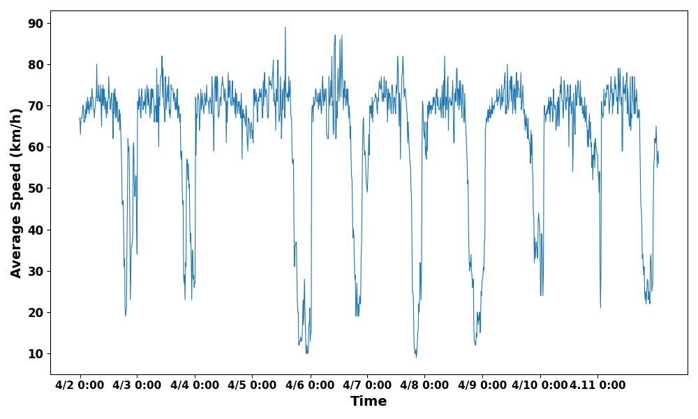
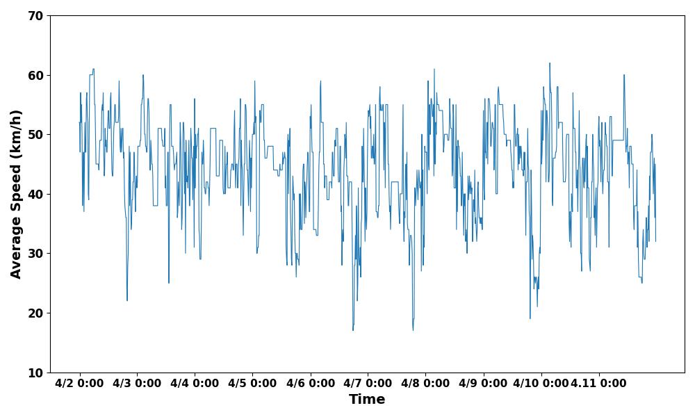
This paper selects two sets of data from the Second Ring Road and Nong Da South Road. They represent the data of main roads and non main roads respectively. These data are the average speeds of vehicles from 0:00 to 10:00 for 10 consecutive days. In order to make the predicted results closer to the true values, a smaller time density division of 5 minutes is selected. Recording the traffic flow information on the road every 5 minutes, so that there are nearly 120 sample values for each day's data. The preliminary timing diagrams of the selected data are shown in Figure 1 and Figure 2.

Figure 1. Average speed of traffic on the Second Ring Road.

Figure 2. Average speed of traffic on Nong Da South Road.

2.3 LSTM method

LSTM is a network model with time cycle as its core, which can better solve the long-term dependence problem of recurrent neural network in operation, that is, gradient disappearance and gradient explosion problems generated in the training process.

The LSTM model consists of three parts: Forest Gate, Input Gate, Output Gate. The Forgotten Gate is responsible for updating the information status, the input gate is responsible for inputting information, while the output gate is responsible for outputting information. In order to realize the function, the LSTM model generally contains repeated modules, as shown in Figure 3. The status between modules can be transferred to each other and run depending on time chain.

Figure 3. LSTM Structure [14].

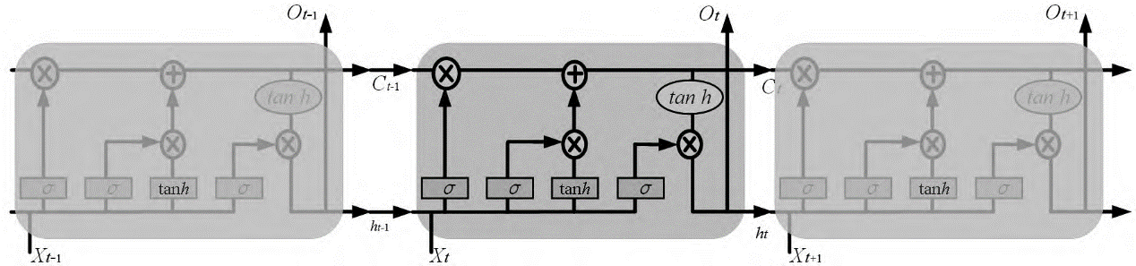
The formula for the forget gate \( f_{t} \) :

\( f_{t} = σ (W_{f} [h_{t-1}, x_{t}]+ b_{f}) \) (2)

The formula for the input gate \( i_{t} \) :

\( i_{t} = σ ⁡(W_{i} [h_{t-1}], x_{t}+b_{i}) \) (3)

\( \widetilde{C}_{t} = tanh ({W_{c}} [h_{t-1}, X_{t}]+b_{c}) \) (4)

The formula for the forget gate \( o_{t} \) :

\( o_{t} = σ (W_{O} [h_{t-1}]+b_{o}) \) (5)

\( h_{t} =o_{t}tanh⁡(c_{t}) \) (6)

\( h_{t-1} \) is the hidden layer state. \( σ \) is the sigmoid nonlinear activation function. \( W \) is the weight between connecting neurons, and \( b \) is the bias of neurons.

2.4 PSO-LSTM method

PSO is an algorithm inspired by the hunting patterns of bird flocks, which utilizes the coordination, cooperation, and information sharing among individuals in a group to find the optimal solution. The process of treating each bird as a particle that constantly moves within a spatial range, with each particle possessing an adaptive velocity and position. The particles in space continuously track and save the optimal particle position by searching for the best position, thus obtaining the global optimal solution.

Firstly, initialize the particle swarm, where each particle represents a possible solution to the problem, focusing on three indicators: fitness, velocity, and position. Through multiple iterations, seek the optimal result. At each iteration, the update of particle velocity and position is based on two optimal solutions, namely individual optimal solution \( pbest \) and population optimal solution \( gbest \) , with the specific formula as follows [15]:

\( v_{i}^{k+1} = v_{i}^{k}+c_{1}r_{1}(pbest_{i}^{k}-x_{i}^{k})+c_{2}r_{2}(gbest^{k}-x_{i}^{k}) \) (7)

\( x_{i}^{k+1} = x_{i}^{k}+v_{i}^{k+1} \) (8)

\( v_{i}^{k+1} \) and \( v_{i}^{k} \) are the velocities of particle \( i \) at the \( k+1 \) th and \( k \) th iterations; \( x_{i}^{k+1} \) and \( x_{i}^{k} \) are the positions of particle \( i \) at the \( k+1 \) th and \( k \) th iterations; \( c_{1} \) and \( c_{2} \) are acceleration factors, where \( c_{1} \) represents the acceleration weight of particles towards the optimal individual position, and \( c_{2} \) represents the acceleration weight of particles towards the optimal group position; \( r_{1} \) and \( r_{2} \) are random numbers within the [0,1].

2.5 Evaluation method

In order to quantitatively evaluate the predictive accuracy of the model, this article selects Mean Squared Error (MSE), root mean squared error (RMSE), and mean absolute percentage error (MAPE) as the evaluation criteria for the model. The expression is:

\( MSE = \frac{1}{n}\sum_{i=1}^{n}(y_{i }-\hat{y_{i}})^{2} \) (9)

\( RMSE = \sqrt[]{\frac{1}{n}\sum_{i=1}^{n}(y_{i }-\hat{y_{i}})^{2}} \) (10)

\( MAPE = \frac{1}{n}\sum_{i=1}^{n}\frac{|y_{i }-\hat{y_{i}}|}{y_{i}} \) (11)

\( n \) is the quantity of data; \( y_{i } \) is the actual value of the data; \( \hat{y_{i}} \) is the predicted value of the data. The smaller the parameter value, the more accurate the prediction result.

3 Results and discussion

3.1 Initial data comparison

Firstly, this paper compares the initial data of the two roads and then draws box plots of both, as shown in Figures 4.

Figure 4. Box plot of two roads.

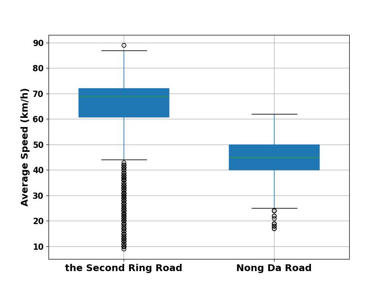
In the boxplot of the Second Ring Road, the rectangular box has a large span and many outliers. The median and mean are relatively high, with large fluctuations and dispersion in the data. In the boxplot of Nong Da South Road, the rectangular box has a smaller span and fewer outliers. The median and mean are relatively low, and the fluctuation and dispersion of the data are small.

The Second Ring Road is a very important main road in Beijing, with a large number of lanes and high traffic volume. However, Nong Da South Road is not adjacent to the main traffic road and has fewer lanes. The two ends of the road are mostly small parks, leisure and entertainment facilities, and the traffic flow is relatively small. Comparing the boxplots, the author can see that the peak speed of vehicles on the Second Ring Road is significantly higher than that on Nong Da South Road, but the lowest value is significantly lower than the average value on Nong Da South Road. This indicates that the road carrying capacity of the Second Ring Road is stronger, but the frequency and impact of morning rush hour are high and significant; The road carrying capacity of Nong Da South Road is relatively weak, but it is less affected by the morning rush hour and the traffic flow is relatively stable.

3.2 LSTM model prediction

After analyzing the data characteristics of both, this paper uses them as datasets and make predictions using an LSTM model. The prediction results of the training set are shown in Figures 5 and 6:

Figure 5. The Second Ring Road prediction result based on LSTM.

Figure 6. Nong Da South Road prediction result based on LSTM.

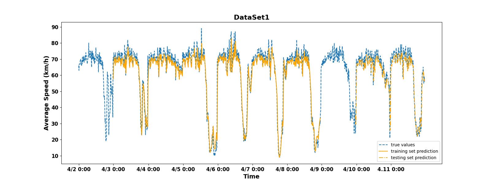
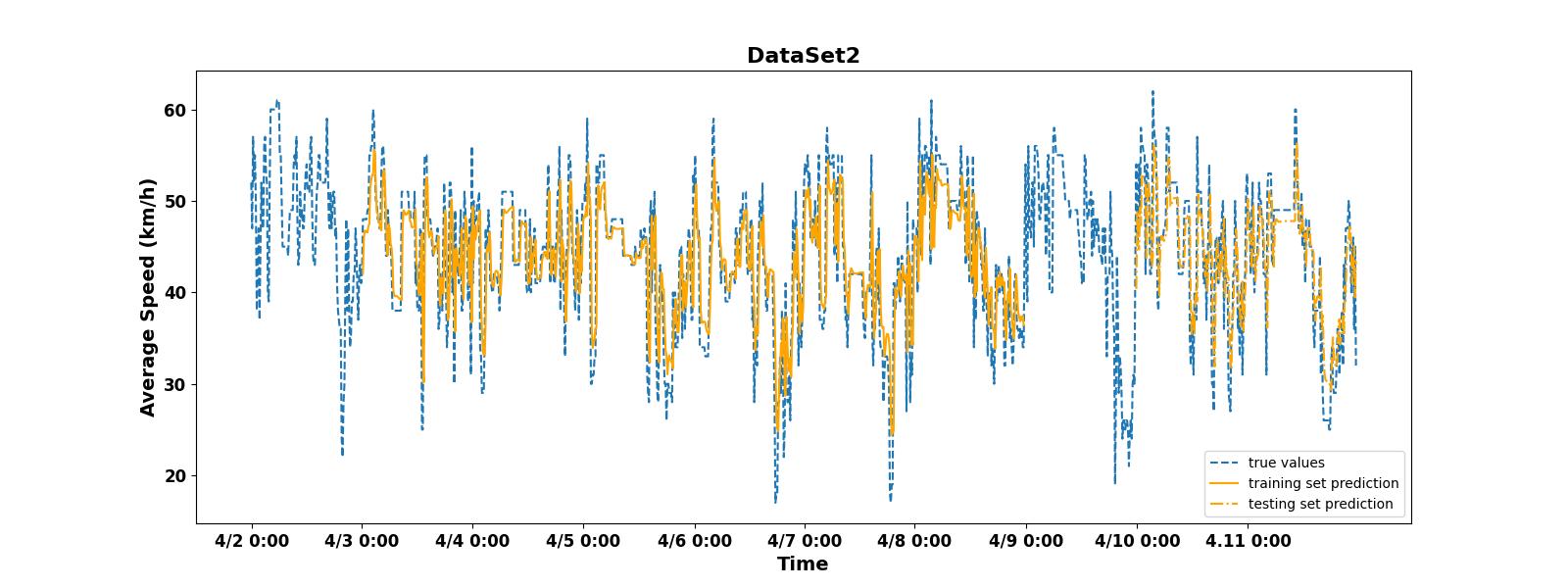
Figure 5 shows that the machine's prediction of the average speed of vehicles on the Second Ring Road is generally consistent. Whether it's the training set or the testing set, the fluctuation and trend of the data are close to the real data. The valley value is almost consistent with the real data. However, there is a slight difference between the peak predicted and the true peak values. The results always seem to be smaller than the true values. Figure 6 shows that the LSTM model also has a relatively accurate prediction result for the second road. The direction of the data fits to the real curve. However, the problem of inaccurate peak prediction also exists. Unlike the previous dataset, the model's prediction of valley values in this dataset is also inaccurate.

There are several reasons that led to the problem of inaccurate valley prediction results in non main road. The dominant factor is whether there is a periodic traffic flow. As a main road, the Second Ring Road is frequently and regularly affected by morning rush hour. This means that the occurrence of valley values in the average driving speed of cars is highly periodic. This pattern can be easily captured and successfully predicted. As a non main road, Nong Da South Road has a low frequency of morning rush hour, so the occurrence of valley values in traffic flow on this road has a high degree of randomness. This will bring greater difficulty to prediction.

Similarly, there are similar reasons why the model's predictions of peak values for both datasets are less accurate. The peak of average speed occurs when the road is relatively idle. Throughout the midnight period, the roads remain relatively empty. This also means that the peak of vehicle will not occur at fixed times, it may randomly appear at some point in the middle of the night. In situations with low traffic flow, any driver driving too fast may affect the occurrence of peak values. This lack of regularity also leads to inaccurate peak prediction in the model.

The correlation statistics of the LSTM model's prediction results for two datasets are shown in Table 1. MSE measures the square of the average error between predicted and actual values. RMSE is the square root of MSE. MSE and RMSE can evaluate the overall prediction accuracy of the model. MAPE measures the percentage of prediction error.

Table 1. Evaluation of LSTM model prediction results

The results indicate that the relevant statistical values of the predicted results of Nong Da South Road are all smaller than those of the Second Ring Road. This means the model performs well for non main road prediction, but relatively poorly for main road prediction. The main factor causing this is the high degree of data dispersion and large outliers in the main road data. The model will be interfered by these outliers when fitting, resulting in poor prediction results. From the results, it can be concluded that the LSTM model has a better prediction effect for data sets with less dispersion.

Overall, the statistics of the prediction results of the evaluation model have reached a low level, the LSTM model produces satisfactory prediction results for both road segments.

3.3 PSO-LSTM model prediction

In order to investigate whether the PSO-LSTM model can make improvements on the basis of the LSTM model, this paper trains the PSO-LSTM model using the same dataset, and the results are shown in Figures 7 and 8.

Figure 7. The Second Ring Road prediction result based on PSO-LSTM

Figure 8. Nong Da South Road prediction result based on PSO-LSTM.

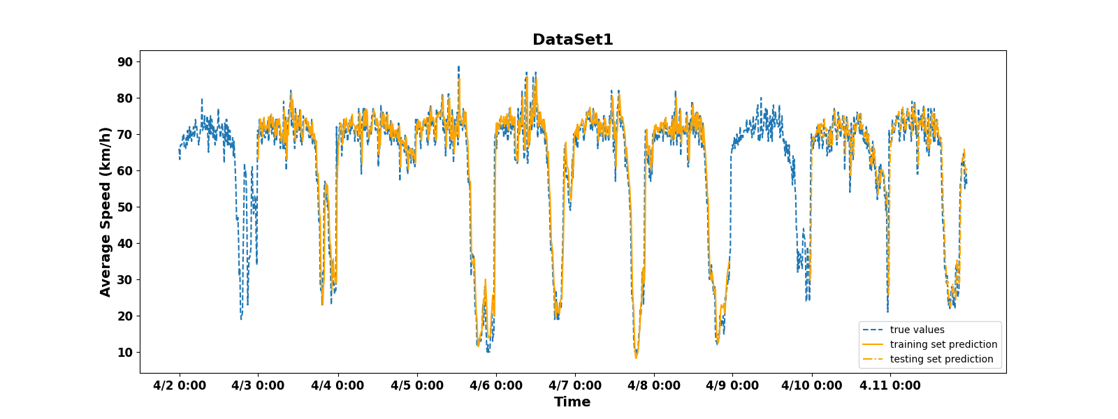
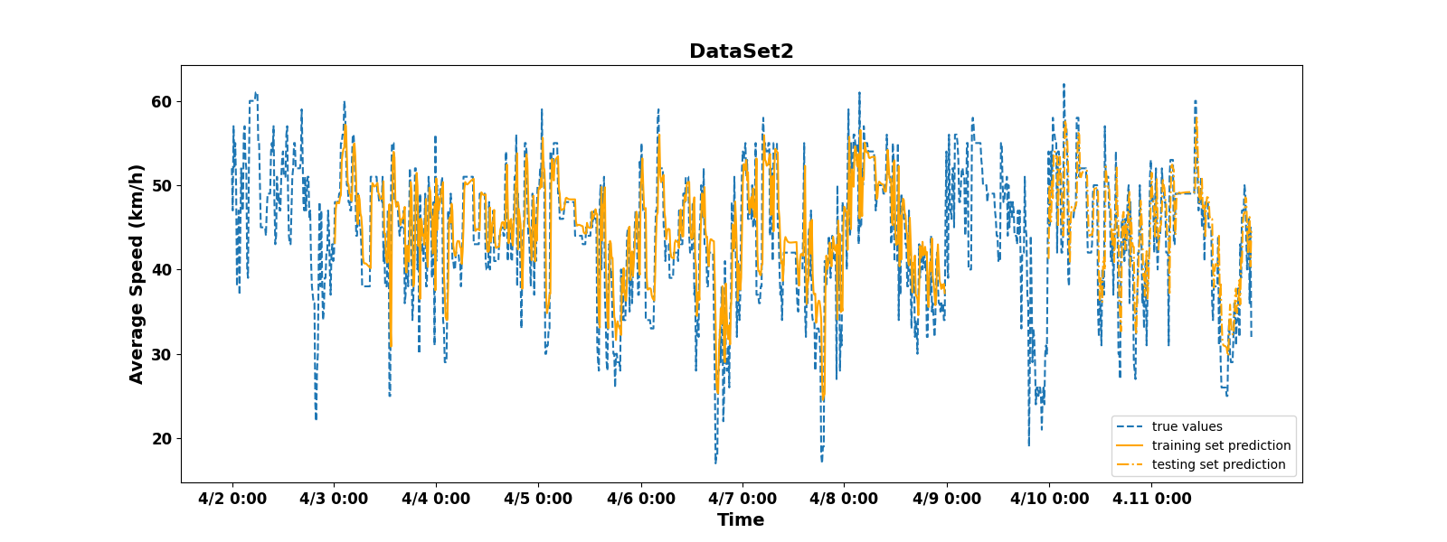
Figures 7 and 8 show that the training results of the PSO-LSTM model are also very satisfactory. In Figure 7, the peak value of the predicted value is quite close to the peak value of the real data, significantly improving the prediction accuracy. In Figure 8, the predicted peak and valley values are also much closer to the true values.

These results indicate that the PSO-LSTM model has to some extent solved the problem of inaccurate prediction of periodic data by LSTM models. This paper also provides the evaluation statistics table for the results of this training, as shown in Table 2.

From Table 2, it can be seen that the relevant statistics of the PSO-LSTM model also maintain a very low value. However, compared to the LSTM model, these statistics do not show significant improvement, and some statistics are even higher than the LSTM model. This indicates that the overall performance of the PSO-LSTM model on this dataset is not better than that of the LSTM model.

Subtracting the statistics of PSO-LSTM dataset 2 from the statistics of dataset 1, and comparing the resulting difference with the difference of the LSTM model. The difference has not lowered, indicating that the PSO-LSTM model still does not improve well in predicting highly discrete data.

Table 2. Evaluation of PSO-LSTM model prediction results

4 Conclusion

This paper aims to research the prediction of traffic flow using an LSTM model. In the study, the average driving speed of road vehicles in Beijing from 0 a.m. to 10 a.m. for 10 consecutive days are selected. The two roads represent the main road that is greatly affected by the morning rush hour and the non main road that is less affected by the morning rush hour. The former has a high degree of data dispersion and many outliers. The latter has a low degree of data dispersion and fewer outliers. The results indicate that the LSTM model has ideal prediction results for both, accurately predicting the trend of the data. Especially, the model has excellent predictive performance for periodic data, but its predictive performance for non periodic data is not satisfying. The model has a higher prediction accuracy for data with low dispersion than for data with high dispersion. Compared to the LSTM model, the PSO-LSTM model has improved the accuracy of predicting non periodic data, but still lacks accuracy in predicting highly discrete data. Subsequent research can attempt to improve the predictive accuracy of the model for non periodic data, while also attempting to reduce the interference of high dispersion and multiple outliers on the model's predictions.

References

[1]. Yang N 2014 Analysis of the hazards and causes of urban traffic congestion. China Market, (42), 100-101.
[2]. Cao C 2020 Research on algorithm of vehicle flow monitoring and prediction based on deep learning. Jimei University.
[3]. Sun H 2020 Research on traffic signal control method based on deep reinforcement learning. Nanjing University.
[4]. Xiang Q 2021 Research on deep reinforcment learning for urban adaptive traffic signal control. Southeast University.
[5]. Shen L, Lu Y and Guo J 2021 Adaptability of Kalman Filter for short-time traffic flow forecasting on national and provincial highways. Journal of Transport Information and Safety. 39(05), 117-27.
[6]. Nihan N L and Holmesland K O 1980 Use of the Box and Jenkins time series technique in traffic forecasting. Transportation, 9(2), 125-143.
[7]. Li T, Ni A, Zhang C, Xiao G and Gao L 2021 Short-term traffic congestion prediction with Conv iLSTM considering spatiotemporal features. IET Intelligent Transport Systems, 14(1).
[8]. Rasheed F, Yau K, and Low Y C 2020 Deep reinforcement learning for traffic signal control under disturbances: A case study on Sunway city Malaysia. Future Generation Computer Systems.
[9]. Smith B L and Demetsky M J 1997 Traffic flow forecasting: comparison of modeling approaches. Journal of transportation engineering, 123(4), 261-266.
[10]. Vanajakshi L and Rilett L R 2004 A comparison of the performance of artificial neural networks and support vector machines for the prediction of traffic speed. IEEE Intelligent Vehicles Symposium. IEEE, 194-199.
[11]. Liu Q, Zhai J, Zhang Z, Zhong S, Zhou Q, Zhang P Xu J 2018 A brief overview of deep reinforcement learning. Chinese Journal of Computers, 1-27.
[12]. Zhang W, Yu Y, Qi Y, Shu F and Wang Y 2019 Short-term traffic flow prediction based on spatiotemporal analysis and CNN deep learning. Transportmetrica, 15(2), 1688-711.
[13]. Zhao M 2021 Prediction for short-term passenger flow of subway based on improved PSO Optimized LSTM neural network. Shijiazhuang Tiedao University.
[14]. Zhu H 2024 Intercity railway passenger flow prediction method based on improved LSTM model. The technology and management of transportation system, 5(13), 4-7.
[15]. Zhang G and Jin H 2021 Passenger flow prediction of urban rail transit stations based on improved PSO-LSTM model. Computer Applications and Software, 3(812), 110-114+134.
Cite this article
Xu,F. (2024). Research on traffic flow prediction method based on LSTM model and PSO-LSTM model. Applied and Computational Engineering,101,154-163.
Data availability
The datasets used and/or analyzed during the current study will be available from the authors upon reasonable request.
Disclaimer/Publisher's Note
The statements, opinions and data contained in all publications are solely those of the individual author(s) and contributor(s) and not of EWA Publishing and/or the editor(s). EWA Publishing and/or the editor(s) disclaim responsibility for any injury to people or property resulting from any ideas, methods, instructions or products referred to in the content.
About volume
Volume title: Proceedings of the 2nd International Conference on Machine Learning and Automation
© 2024 by the author(s). Licensee EWA Publishing, Oxford, UK. This article is an open access article distributed under the terms and
conditions of the Creative Commons Attribution (CC BY) license. Authors who
publish this series agree to the following terms:
1. Authors retain copyright and grant the series right of first publication with the work simultaneously licensed under a Creative Commons
Attribution License that allows others to share the work with an acknowledgment of the work's authorship and initial publication in this
series.
2. Authors are able to enter into separate, additional contractual arrangements for the non-exclusive distribution of the series's published
version of the work (e.g., post it to an institutional repository or publish it in a book), with an acknowledgment of its initial
publication in this series.
3. Authors are permitted and encouraged to post their work online (e.g., in institutional repositories or on their website) prior to and
during the submission process, as it can lead to productive exchanges, as well as earlier and greater citation of published work (See
Open access policy for details).