1.Introduction

Recent years have seen a tremendous increase in the market need for sophisticated autonomous driving systems due to the development of new energy vehicles. However, current self-driving cars still face many technical challenges, among which obstacle detection and trajectory prediction in dynamic environments is one of the main difficulties. Recent years have seen a rapid development of deep learning techniques, which have shown significant promise in several disciplines such massive language modeling and computer vision. Yao et al.'s multimodal deep learning framework achieved a technological breakthrough and opened up new research areas [1]. In addition, many novel network models [2] provide new ideas and methods for obstacle recognition and trajectory prediction in intelligent driving systems. The following are a few popular deep learning techniques for intelligent driving systems' obstacle detection and trajectory prediction.

In recent years, the technology of autonomous driving systems has advanced rapidly due to the development of various machine learning and deep learning approaches. Convolutional neural networks (CNN) are a key component of computer vision and image processing, and they are extensively utilized in self-driving systems. Through CNN, the vehicle can recognize the features of the road and obstacles captured by the camera in real time, significantly improving the environmental awareness of autonomous vehicles. This year's research on CNN focuses on how to optimize the architecture and algorithm of CNN, and improve the accuracy and speed of image recognition [3]. Recurrent neural networks (RNN) and their improved versions, Long Short-Term Memory (LSTM), work incredibly well when building temporal models. While LSTM uses a gating mechanism to address the gradient disappearance issue with regular RNNs, RNN is capable of capturing order dependence in time series data. The main applications of these technologies in autonomous driving are trajectory prediction and behavior analysis [4]. To handle complicated driving scenarios, researchers are attempting to increase these models' processing speed and forecast accuracy [5].

These are some additional deep learning techniques that are essential to autonomous vehicle systems. Reinforcement Learning (RL) and Deep Reinforcement Learning (DRL) technologies improve the adaptiveness of the autonomous driving system in terms of control and decision-making through a mechanism of trial and error and strategy optimization. Current research focuses include how to efficiently train RL models in high and dynamic environments, and how to combine deep learning techniques to enhance the processing power of the models [6]. Simultaneous Localization and Mapping (SLAM) technology also plays a crucial part in autonomous driving. Multimodal sensor fusion technology significantly improves the sensing accuracy and robustness of autonomous driving systems in complex environments by integrating data from different sensors [7]. SLAM integrates this data to enable real-time positioning and mapping of vehicles in unknown environments. Researchers are continuously optimizing SLAM algorithms to improve their robustness and accuracy in dynamic and complex environments [8].

To improve self-driving cars' ability to recognize obstacles in real time and anticipate their course in changing conditions, this paper proposes an obstacle recognition and trajectory prediction model that combines a GRU network with a 3D CNN. The model makes use of the advantages of GRU in time-series data prediction and the potent feature identification power of 3D CNN to precisely detect and predict the course of dynamic obstacles, thereby improving the performance of the autonomous driving system in different complex environments. For example, in the application of visual SLAM (simultaneous localisation and map building) technology, the integrated framework is able to process real-time sensory data more efficiently, providing more accurate environmental maps and localisation information.

In this paper, the research validates the significant advantages of the proposed method for dynamic obstacle recognition and prediction through experiments on publicly available datasets such as KITTI and Argoverse. The system outperforms existing approaches not just in terms of identification and prediction accuracy but also in terms of total model operating efficiency, as demonstrated by experimental results. These results imply that a realistic and efficient approach that can strongly promote the advancement of autonomous driving technology is an obstacle recognition and trajectory prediction model that combines GRU with 3D CNN.

After that, this paper will go into great length on the suggested model's technical specifications, experimental design, and result analysis. It will also go over the possibility of using this model in the autonomous driving space.

2.Methodology

2.1.Overview

The technology aims to integrate GRU and 3D CNN methods for effective obstacle identification and trajectory prediction in self-driving cars. The technique addresses crucial elements like obstacle and object identification to raise the autonomy and security of self-driving cars. Figure 1 illustrates a summary of the flow of the model:

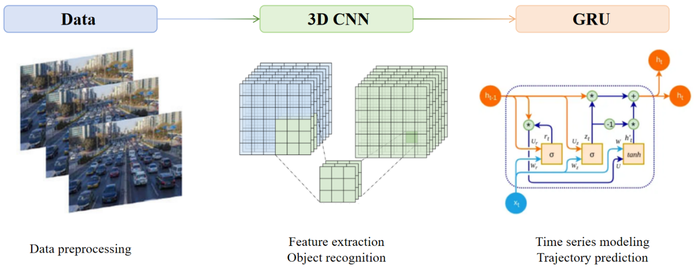
In general, the techniques described in this work are used through time series modeling, dynamic obstacle trajectory prediction, object recognition and feature extraction, and data processing. After selecting the dataset's data at random for processing, 3D CNN is used to extract spatiotemporal characteristics for object and obstacle recognition from environmental image sequences. In order to precisely identify barriers in real time, the model learns from various objects in the environment and extracts their properties. The trajectory and behavior of the dynamic obstacles are then modeled by the GRU model using the 3D CNN extracted feature sequences as input. By learning past data, the GRU can forecast the movement trajectory of obstacles, hence reducing the probability of collision in the ensuing path planning system. Through the above process, the model can realize the obstacle identification and trajectory prediction in the self-driving system, improve the identification efficiency of the system, lower the operational risk and offer a helpful resource for future technical advancements in the area of self-driving automobiles.

2.2.D Convolutional Neural Network

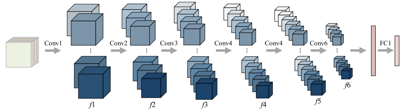
An extension of the conventional 2D CNN, the 3D CNN is a deep learning model that excels in processing 3D data, such as video and medical pictures. 3D CNN is able to record the temporal and spatial properties of the data since it can perform convolutional operations in both temporal and spatial dimensions. It is extensively employed in the domains of behavioral recognition, medical image analysis, video analysis, and so on. It is capable of efficiently extracting and utilizing multi-dimensional data to enhance the model's accuracy [9]. The primary distinction between 2D and 3D CNN is the size and convolved nature of the data being processed. 2D CNN processes two-dimensional data (e.g., still images) with a convolution kernel that slides only in a two-dimensional plane and convolves only in the spatial dimension. Whereas 3D CNN processes three-dimensional data, its convolution kernel slides in three-dimensional space, not only in the spatial dimension, but also in the temporal dimension, thus capturing both spatial as well as temporal dynamic information. This allows 3D CNN to perform better in dynamic environments where temporal variations need to be taken into account, such as video classification and action recognition. As shown in Figure 2 and Figure 3, the two pictures show the 3D convolution process and the model structure of 3D CNN.

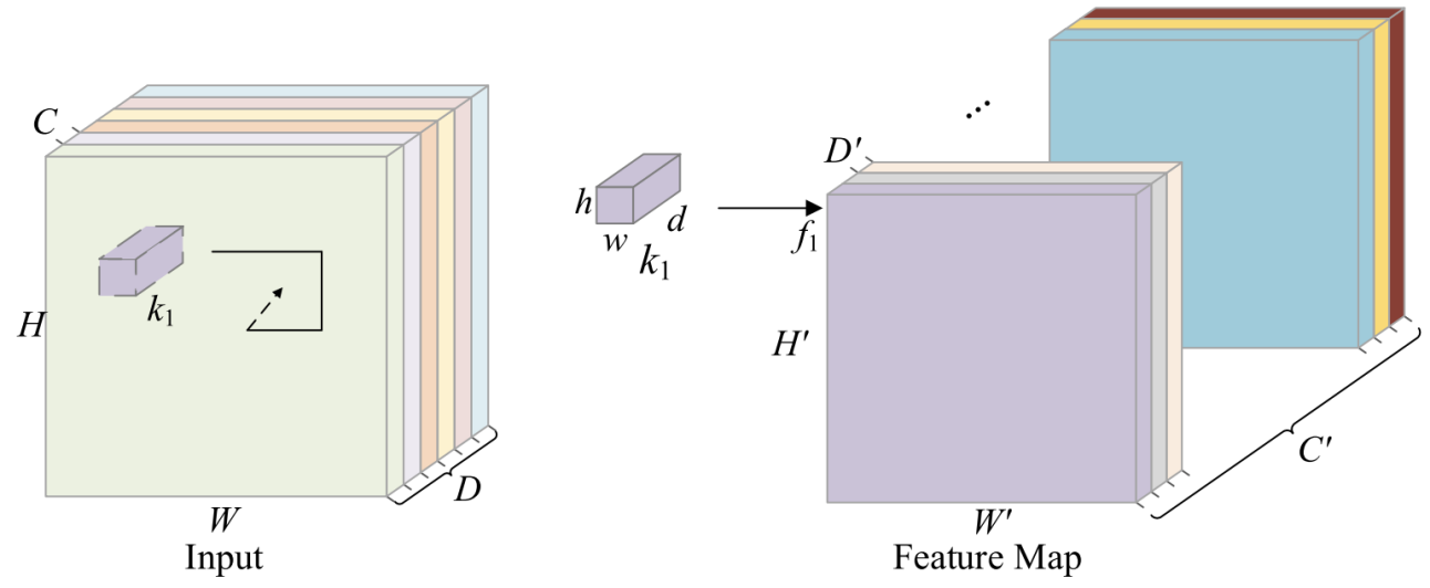
Figure 2. Diagrammatic representation of the 3D convolution process.[10]

Three popular 3D CNN formulations and their varying interpretations are listed below [11].

\( {Y_{i,j,k}}=\sum _{m=1}^{M}\sum _{n=1}^{N}\sum _{l=1}^{L}{X_{i+m,j+n,k+l}}∙{W_{m,nl}} \)(1)

\( {Y_{i,j,k}} \): Provide the feature map's value at the specified place (i, j, k)

X: Input feature map

W: Convolutional kernel with three dimensions M, N and L

\( \sum _{m=1}^{M}\sum _{n=1}^{N}\sum _{l=1}^{L} \): summing over all elements of the convolution kernel

\( {X_{i+m,j+n,k+l}} \): the value of the local region of the input feature map that matches the convolution kernel

\( {W_{m,nl}} \): Weights of the convolution kernel at positions (m, n, l).

\( {Y_{i,j,k}}=m_{m=1}^{M}m_{n=1}^{N}m_{l=1}^{L}{X_{i+m,j+n,k+l}} \)(2)

\( {Y_{i,j,k}} \): values for the feature map's output at those locations (i, j, k)

\( {X_{i+m,j+n,k+l}} \): Put the volume's components in at (i+m, j+n, k+l) places.

max: Maximum pooling operation that takes the maximum value in a local region.

m,n,l: indicates the width, height, and depth dimensions of the convolution kernel index.

M, N, L: describes the convolution kernel's width, height, and depth dimensions.

\( {Y_{i,j,k}}=f(\sum _{m=1}^{M}\sum _{n=1}^{N}\sum _{l=1}^{L}{X_{i+m,j+n,k+l}}∙{W_{m,nl}}+b) \)(3)

\( {Y_{i,j,k}} \): Output values for the feature map at those places (i, j, k)

\( {X_{i+m,j+n,k+l}} \): the value of the local region of the input feature map that matches the convolution kernel

\( {W_{m,nl}} \): the value of the input feature map's local region matching the convolution kernel

b: biased phrase

\( f \): activation mechanism

\( \sum _{m=1}^{M}\sum _{n=1}^{N}\sum _{l=1}^{L} \): summing over all elements of the convolution kernel

M, N, L: describes the convolution kernel's width, height, and depth dimensions.

2.3.Gated Recirculation Unit (GRU)

GRU networks differ from LSTM networks due to their less complicated structure. GRU is a sort of RNN architecture designed to handle short-term memory difficulties. GRU converts the input and oblivion gates of the LSTM into a single update gate, resulting in a structural architecture that is more straightforward. Additionally, GRU lacks a distinct unit state, in contrast to LSTM.

The update gate, reset gate, and current memory contents make up the three primary components of the GRU unit. By employing these gates, the GRU may discern long-term dependencies within the sequence by selectively updating and utilizing data from previous time steps. The GRU unit's structure is shown in Figure 4.

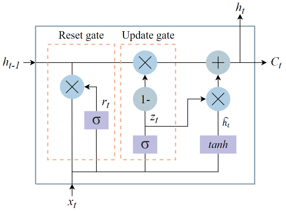
The following is a brief description of the GRU unit structure:

•Update the door:

\( {z_{t}}=σ({W_{r}}[{h_{t-1}},{x_{t}}]+{b_{r}}) \)(4)

How much historical data should be kept and integrated with the present input is decided by the update gate. The output is produced by concatenating the prior hidden state with the current input using a sigmoid activation function and a linear transformation.

•Reset the door:

\( {r_{t}}=σ({W_{r}}[{h_{t-1}},{x_{t}}]+{b_{r}}) \)(5)

The reset gate establishes the threshold for erasing historical data. It uses the output of the previous hidden state and the current input consecutively to calculate in a manner akin to an update gate.

•Current memory content:

\( \widetilde{{h_{t}}}=tanh({W_{h}}[{r_{t}}{h_{t-1}},{x_{t}}]) \)(6)

The current memory content is determined by the reset gate and the concatenation of the previous concealed state with the current input; candidate activations are generated by a hyperbolic tangent activation function.

•Final memory state:

\( {h_{t}}=(1-{z_{t}}){h_{t-1}}+{z_{t}}\widetilde{{h_{t}}} \)(7)

The final memory state is determined by the combination of the candidate activation and the previous concealed state, and the update gate controls the proportion between the two.

•Output Gate:

\( {o_{t}}={σ_{o}}({W_{o}}{h_{t}}+{b_{o}}) \)(8)

Output gates control the information flow from the contents of the current memory to the output; these gates are usually computed using a sigmoid activation function.

Compared to LSTM, GRU has the benefits of a simpler structure, more computational efficiency, and a smaller memory demand. GRU reduces the parameters and computational steps and improves the training speed by merging the input and forgetting gates into an update gate. Meanwhile, GRU can provide similar performance to LSTM in many tasks, but is more efficient and suitable for application scenarios with limited computational resources.

3.Description of the experiment

3.1.Datasets

The study conducted in this paper largely uses the following two datasets for model training and evaluation:

•A sizable dataset for assessing technology related to computer vision and autonomous driving is the KITTI dataset. The Toyota Technological Institute and the Karlsruhe Institute of Technology developed it. This dataset's data were gathered from real-world urban traffic situations. High-resolution photos, LiDAR point clouds, GPS and IMU data, and 3D target labeling are all included in the dataset. The KITTI dataset is widely used for research in visual perception, object detection, tracking, stereo vision, depth estimation, and other tasks, and is a valuable asset in the realm of driverless vehicles. The following links will allow you to obtain certain datasets and data items: http://www.cvlibs.net/datasets/kitti

•Argo AI launched the Argoverse dataset, a big dataset devoted to research on autonomous driving. It contains detailed sensor data and high-precision maps, and the dataset is designed to facilitate the development of autonomous driving technology. The Argoverse dataset includes synchronised data collected by multi-sensor platforms (e.g. cameras, LiDAR), 2D and 3D object annotations, trajectory prediction, and lane centreline information. The Argoverse 3D tracking dataset and the Argoverse motion prediction dataset comprise the two primary sections of the dataset. It is extensively utilized in the creation and assessment of algorithms for perception, prediction, and planning in autonomous driving. Specific data content and dataset downloads can be accessed at the links below: https://www.argoverse.org

3.2.Experimental details

Two datasets are chosen for training in this work, and the training outcomes are as follows:

3.2.1.Data processing. In this paper, scenarios of autonomous vehicles functioning in various settings are simulated and trained using multiple medium data types such as scene images, point cloud data, and sensor data from KITTI and Argoverse.

3.2.2.Feature extraction and obstacle type recognition. In this work, the researchers recognize barrier species and extract temporal information from image sequences using 3D CNN. Firstly, this model feeds video or continuous frame data into the 3D CNN model, with each input containing multiple continuous frames. A 3D convolutional kernel is applied in both temporal and spatial dimensions in order to extract the spatial characteristics of each frame as well as the temporal aspects between frames. Multi-layer 3D convolution and pooling operations progressively refine the high-level features, and finally the obstacle classification is performed through a fully connected layer that outputs the probability of each obstacle class using the Softmax function.

3.2.3.Forecasting the trajectory of obstacles and time-series modeling. The goal of this experiment is to anticipate obstacle trajectories and model time series using a model that combines a 3D CNN and a GRU. To precisely forecast the paths of obstacles in dynamic situations, the model makes use of the spatial feature extraction capabilities of 3D CNN and the time-series processing capabilities of GRU.

The model structure includes 3D CNN module and GRU module. Spatial features are extracted from the input continuous frame image using the 3D CNN module. The input data is a series of image frames that are preprocessed to form a 3D tensor (T represents the number of time steps, H and W stand for the picture's width and height, and C stands for the number of channels. The result is T × H × W × C). The 3D CNN module consists of three 3D convolutional layers and three 3D pooling layers. A ReLU activation function comes after each convolutional layer. The specific structure is as follows:

1st 3D convolutional layer: convolutional kernel size is 64×64×64×3;

1st pooling layer: Step size is 2×2×2, and pooling window size is 2×2×2;

2nd 3D convolutional layer: convolutional kernel size of 32 × 32 × 32 × 32;

2nd pooling layer: Step size is 2×2×2, and pooling window size is 2×2×2;

The 3rd 3D convolutional layer: convolutional kernel size of 16 × 16 × 16 × 64;

3rd pooling layer: Step size is 2×2×2, and pooling window size is 2×2×2;

The 4th 3D convolutional layer: convolutional kernel size of 8 × 8 × 8 × 128;

The output features of the convolutional layer are then passed to the fully connected layer 1, which has an output dimension of 512, using the ReLU activation function once again after being split up into one-dimensional vectors by a flatten layer. Lastly, the output dimension of the fully linked layer 2 and the total number of output categories in the task are often equal.

The spatio-temporal feature sequences after performing 3D CNN processing are input into the GRU model for temporal modelling and obstacle trajectory prediction. To model the time series properties, the research input these feature vectors into the GRU module. It is made up of two GRU modules. The ReLU activation function is used to activate the first entirely linked layer with an output size of 128. The output dimension of the fully connected layer 2 is 256. The loss function and optimizer to be utilized in the GRU model depend on the specific task. Typically, the optimizer selects the mean square error loss function and employs Adam with a learning rate of 0.001.

3.2.4.Conclusion. The following procedures are involved in the entire experiment: data processing, dynamic obstacle trajectory prediction, time series modeling, feature extraction, and obstacle species identification. By utilizing these models, self-driving cars can effectively leverage deep learning techniques and multimodal data to perform real-time obstacle recognition and trajectory prediction.

The following will explain the evaluation formulas in is experiment:

•Training time:

\( Training Time=Finish Time-Begin Time \)(9)

•Projected losses:

\( Predict Loss=\frac{1}{N}\sum _{i=1}^{N}{({y_{i}}-\hat{{y_{i}}})^{2}} \)(10)

N: sample size

\( {y_{i}} \): the I sample's actual value

\( \hat{{y_{i}}} \): predicted value for sample i

\( {({y_{i}}-\hat{{y_{i}}})^{2}} \): squared error for the i sample between the true and anticipated values

•Parameters:

\( Parameters=Number of Parameters \)(11)

3.3.Experimental results and analysis

The study's experimental findings will be analyzed, and this model will be compared with other existing models to show the advantages and characteristics of this model.

Figure 5 shows the loss epoch curve and accuracy epoch curve for training and validation. It is evident that the model has quickly trained to reach high accuracy and polar loss value.

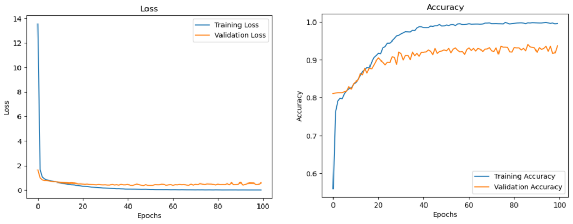
Figure 5. Loss epoch curves and accuracy epoch curves for training and validation

In Table 1, Figure 6 and Figure 7, the performance of CNN-LSTM [12], UB-LSTM [13] and CNN-BiLSTM [14] as well as 3D CNN-GRU models are compared using several datasets (KITTI, Argoverse) in terms of training time, prediction loss, and parameters.

The term “parameters” refers to the quantity of parameters in the model. A simpler and more broadly applicable model is typically associated with fewer parameters. Table 1 shows that the 3D CNN-GRU model has very few parameters, suggesting that our approach is more efficient and has the potential to be more widely applied.

The amount of time the model needs to finish each training cycle is called the training time. In application scenarios of autonomous driving systems, shorter training times are crucial. The information in the table shows that the 3D CNN-GRU model's training time on each dataset is noticeably less than that of the other models, suggesting that our model can effectively increase training speed and is appropriate for self-driving car applications in the real world.

The prediction loss indicates how well the obstacle recognition and trajectory prediction models work. The capacity of the model to correctly identify and forecast the course of an obstacle is shown by a smaller prediction loss. 3D CNN-GRU has a low prediction loss on both models, as demonstrated by the information in Table 1, indicating that our model maintains a good recognition and prediction accuracy even with the suggested reduction in training time.

Table 1. A rather more intricate table with a brief description.

4.Discussion

4.1.Summary of Strengths

This work proposes a GRU and 3D CNN obstacle recognition and trajectory prediction model that has some noteworthy advantages:

•High-precision recognition: because 3D CNN is used for feature extraction of image sequences, this model is able to recognise obstacles efficiently even in complex dynamic environments. The experiment's results show that the model's accuracy in identifying obstacles is far higher than that of traditional methods.

•Accurate Prediction: The GRU model can use historical data for time series prediction, thus providing accurate prediction of the movement trajectory of obstacles. Combined with the feature sequences extracted by the 3D CNN, the GRU can more accurately capture the behavioural patterns of dynamic obstacles and accurately predict obstacle trajectories.

•Efficient processing: the method proposed in this study excels in terms of efficiency of model runs. The model maintains excellent accuracy while drastically reducing computing complexity and speeding up model execution. This improvement is particularly important for autonomous driving systems with high real-time requirements.

•High generality: the model performs well on different types of datasets in the test results, proving its generality and robustness in different environments.

4.2.limitations analysis

Although the present model has achieved some results in obstacle identification and trajectory prediction, there are still some limitations:

•Data dependency: The quantity and quality of training data have a major impact on the model's performance. The model's ability to adjust to novel circumstances may be hampered by inadequate or skewed training data.

•Handling of complex environments: although the present model performs well in most cases, in extremely complex environments (e.g., bad weather, nighttime, etc.), the degree of recognition and prediction accuracy declines significantly.

•Demand for computational resources: Despite the fact that this paper has maximized the model's computational efficiency, the high computational complexity of 3D CNN and GRU itself means that there is still a significant demand for computational resources in real-world applications, which could make it difficult to use the model on autonomous driving systems.

4.3.Improvement programme

To address the above limitations, the following improvement options can be considered for future research:

•Data Enhancement: boost the variety and richness of training data using data augmentation strategies (e.g., data synthesis, data extension, etc.) to strengthen the model's capacity to generalize across various contexts.

•Model optimisation: further optimise the structure of 3D CNNs and GRUs, and adopt lightweight models (e.g. MobileNet, TinyGRU, etc.) in order to reduce the demand for computational resources while maintaining high recognition and prediction accuracy.

•Multi-sensor fusion: fusing data from other sensors, such as LiDAR and millimetre-wave radar, with vision data to build a more comprehensive environment perception model, which in turn improves recognition and prediction capabilities in complex environments.

5.Conclusion

In this study, an obstacle recognition and trajectory prediction model combining 3D CNN and GRU is proposed, and its ability to efficiently recognise obstacles and predict their trajectories in dynamic environments is experimentally verified. The method has high operational efficiency and high versatility while improving accuracy and precision. Despite limitations such as data dependency, complex environment processing capability and computational resource requirements, the performance of the model and its application prospects can be further enhanced by improvement schemes such as data augmentation, model optimisation and multi-sensor fusion.

The experiment's findings highlight the value of an integrated framework that includes 3D CNNs and GRUs in the development of autonomous driving technology since it can provide autonomous driving systems with safer and more intelligent solutions. Future research will continue to explore more efficient model structures and optimisation methods to facilitate the further development and application of autonomous driving technologies.

References

[1]. Yao, J., Zhang, B., Li, C., Hong, D., & Chanussot, J. (2023). Extended vision transformer (ExViT) for land use and land cover classification: A multimodal deep learning framework. IEEE Transactions on Geoscience and Remote Sensing, 61, 1-15.
[2]. Taye, M. M. (2023). Theoretical understanding of convolutional neural network: Concepts, architectures, applications, future directions. Computation, 11(3), 52.
[3]. Salehi, A. W., Khan, S., Gupta, G., Alabduallah, B. I., Almjally, A., Alsolai, H., ... & Mellit, A. (2023). A study of CNN and transfer learning in medical imaging: Advantages, challenges, future scope. Sustainability, 15(7), 5930.
[4]. Shiri, F. M., Perumal, T., Mustapha, N., & Mohamed, R. (2023). A comprehensive overview and comparative analysis on deep learning models: CNN, RNN, LSTM, GRU. arXiv preprint arXiv:2305.17473.
[5]. Li, S. E. (2023). Deep reinforcement learning. In Reinforcement learning for sequential decision and optimal control (pp. 365-402). Singapore: Springer Nature Singapore.
[6]. Liu, Y., Lu, Y., Nayak, K., Zhang, F., Zhang, L., & Zhao, Y. (2022, November). Empirical analysis of eip-1559: Transaction fees, waiting times, and consensus security. In Proceedings of the 2022 ACM SIGSAC Conference on Computer and Communications Security (pp. 2099-2113).
[7]. Huang, K., Shi, B., Li, X., Li, X., Huang, S., & Li, Y. (2022). Multi-modal sensor fusion for auto driving perception: A survey. arXiv preprint arXiv:2202.02703.
[8]. Ebadi, K., Bernreiter, L., Biggie, H., Catt, G., Chang, Y., Chatterjee, A., ... & Carlone, L. (2023). Present and future of slam in extreme environments: The darpa subt challenge. IEEE Transactions on Robotics.
[9]. Elbaz, K., Shaban, W. M., Zhou, A., & Shen, S. L. (2023). Real time image-based air quality forecasts using a 3D-CNN approach with an attention mechanism. Chemosphere, 333, 138867.
[10]. Wang, P., Wang, P., Wang, C., Xue, B., & Wang, D. (2022). Using a 3D convolutional neural network and gated recurrent unit for tropical cyclone track forecasting. Atmospheric Research, 269, 106053.
[11]. Ma, X., Man, Q., Yang, X., Dong, P., Yang, Z., Wu, J., & Liu, C. (2023). Urban feature extraction within a complex urban area with an improved 3D-CNN using airborne hyperspectral data. Remote Sensing, 15(4), 992.
[12]. Tay, N. C., Tee, C., Ong, T. S., & Teh, P. S. (2019, November). Abnormal behavior recognition using CNN-LSTM with attention mechanism. In 2019 1st International Conference on Electrical, Control and Instrumentation Engineering (ICECIE) (pp. 1-5). IEEE.
[13]. Xiao, H., Wang, C., Li, Z., Wang, R., Bo, C., Sotelo, M. A., & Xu, Y. (2020). UB‐LSTM: a trajectory prediction method combined with vehicle behavior recognition. Journal of Advanced Transportation, 2020(1), 8859689.
[14]. Halder, R., & Chatterjee, R. (2020). CNN-BiLSTM model for violence detection in smart surveillance. SN Computer science, 1(4), 201.
Cite this article
Wang,Z. (2024). Advanced obstacle recognition and trajectory prediction for autonomous vehicles using 3D CNN and GRU. Applied and Computational Engineering,101,164-174.
Data availability
The datasets used and/or analyzed during the current study will be available from the authors upon reasonable request.
Disclaimer/Publisher's Note
The statements, opinions and data contained in all publications are solely those of the individual author(s) and contributor(s) and not of EWA Publishing and/or the editor(s). EWA Publishing and/or the editor(s) disclaim responsibility for any injury to people or property resulting from any ideas, methods, instructions or products referred to in the content.
About volume
Volume title: Proceedings of the 2nd International Conference on Machine Learning and Automation
© 2024 by the author(s). Licensee EWA Publishing, Oxford, UK. This article is an open access article distributed under the terms and
conditions of the Creative Commons Attribution (CC BY) license. Authors who
publish this series agree to the following terms:
1. Authors retain copyright and grant the series right of first publication with the work simultaneously licensed under a Creative Commons
Attribution License that allows others to share the work with an acknowledgment of the work's authorship and initial publication in this
series.
2. Authors are able to enter into separate, additional contractual arrangements for the non-exclusive distribution of the series's published
version of the work (e.g., post it to an institutional repository or publish it in a book), with an acknowledgment of its initial
publication in this series.
3. Authors are permitted and encouraged to post their work online (e.g., in institutional repositories or on their website) prior to and
during the submission process, as it can lead to productive exchanges, as well as earlier and greater citation of published work (See
Open access policy for details).