1. Introduction

2020 saw a dramatic shift in higher education around the globe owing to the COVID-19 pandemic, which pushed universities to quickly switch to online instruction [1]. So, MOOCs emerged as a result. While Massive Open Online Courses (MOOC) can serve several students of all ages simultaneously, it is not without its drawbacks. A severe issue is the absence of prompt feedback regarding instruction. It is challenging for professors to determine whether students have understood the material by traditional techniques because they are unable to observe students' facial expressions and activities on the majority of online learning platforms [2]. At this point, a new way is required to provide feedback to teachers, allowing them to clarify whether students are confused about the knowledge points being taught, and then adjust the teaching progress accordingly. The human brain's impulses can be captured by Electroencephalography (EEG), which holds enormous promise for the analysis of brain activity and conditions [3]. New solutions have also been proposed for feedback.

Machine learning (ML)is the capacity of computers to automate the process of building analytical models and completing related activities by learning from training data specific to a given situation. Machine learning has come a long way in the last few decades, particularly in terms of sophisticated learning algorithms and efficient pre - processing techniques [4]. At the moment, a variety of scientific, engineering, and research domains assess and employ Brain-Computer Interface (BCI) to create applications that offer answers to challenging issues [5]. Machine learning is also applied to various medical diagnoses, such as deep venous thrombosis [6]. Deep learning is a machine learning paradigm based on artificial neural networks [4]. Deep neural networks perform better than machine learning methods for the bulk of the text, image, audio, voice, and video processing techniques because fields with huge and high-dimensional data benefit from the usage of DL. However, machine learning algorithms can still produce better results for low-dimensional data input, particularly when there is not enough training data. These results are even easier to understand than those of deep neural networks [7].

Therefore, combining EEG signals with machine learning is currently a more effective way to classify students' confused states [8]. The current level of student confusion and non-confused state classification is achieved by four distinct machine learning models, with an average classification accuracy of 74% [9]. Therefore, improving the precision of artificial intelligence models is currently necessary. This study compared six many models of machine learning and found that the XGB model was significantly better than other models with an accuracy of 99.69%, greatly improving the classification accuracy of students' confused and non-confused states.

2. Methods

2.1. Dataset

The dataset has prepared 20 videos, 10 of which are thought to be online educational videos that won't confuse college students. These include videos on topics like quantum mechanics and stem cell research, as well as videos introducing basic algebra and geometry. Each video is about 2 minutes long, with two minutes of clips cut out to make the topic more confusing. Normal college students could be confused by these ten videos. A wireless MindSet with a single channel that measures frontal brain activity is worn by the students. MindSet measures the voltage between the ground and the reference electrodes, two electrodes—that are in contact with the ears and an electrode that is placed on the forehead. Ten pupils who have each seen ten videos have had their data collected. The dataset consists of: Predefinedlabel, user-definedlabel, SubjectID, VideoID, Attention, Mediation, Raw, Delta, Theta, Alpha1, Alpha2, Beta1, Beta2, Gamma1, Gamma2 [10].

2.2. Data processing

To effectively manage the dataset for machine learning, this work employs the SimpleImputer with the mean imputation strategy to handle the limited missing values, thereby preserving valuable data that might otherwise be lost through row or column deletion. The visualization results are demonstrated in Figure 1 and Figure 2. The author also converts categorical variables such as gender, ethnicity, and VideoID into numerical representations to make them suitable for machine learning algorithms. Additionally, to lessen the impact of outliers on the functionality of the model, this work applies value capping to the numerical features at the 1st and 99th percentiles. Then, divided the collection into subsets according to the labels that the user has defined, ensuring that the data is organized for targeted analysis and modeling.

Despite ‘VideoID’ having significant information gain, it is excluded to prevent the model from overfitting to IDs and to ensure focus on essential attributes. The most important features are [‘Gamma1’, ‘Alpha2’, ‘Delta’, ‘Beta1’, ‘Alpha1’, ‘Theta’, ‘Attention’, ‘Gamma2’, ‘Beta2’, ‘SubjectID’, ‘Raw’, ‘age’, ‘predefinedlabel’, ‘Mediation’, ‘ethnicity’, ‘gender’]. To normalize the features, they are scaled to have a mean of 0 and a standard deviation of 1. Next, an 80/20 split of the dataset is made into training and test sets.

Figure 1. Distributions of features in the dataset (Figure Credits: Original).

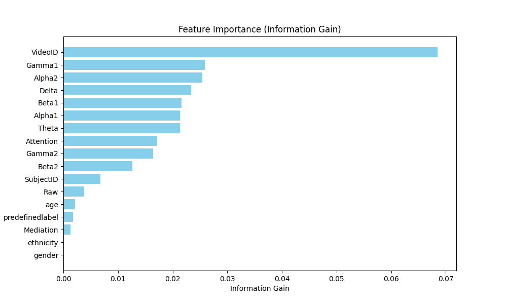
Figure 2. Feature importance in the dataset (Figure Credits: Original).

2.3. Machine learning models

2.3.1. eXtreme Gradient Boosting (XGB). XGB is a type of boosting algorithm that has demonstrated success in numerous domains. It combines several learning algorithms to produce a prediction performance that is superior to any one of the component learning algorithms alone. In contrast to the conventional Gradient Boosting Decision Tree (GBDT) approach, XGB concurrently implements the first and second derivatives and fits the loss function with a second-order Taylor expansion. Moreover, a regularization term is included in the goal function to lessen its complexity and enhance the generalizability of a single tree. To put it briefly, XGB has drawn interest from researchers because of its quick speed, superior classification performance, and support for bespoke loss functions [11].

2.3.2. Random Forest (RF). Combining various tree predictors results in a random forest where each tree depends on the values of a randomly sampled random vector with the same distribution for each tree. As the number of trees in a forest increases, the generalization error approaches a limit. The strength of each individual tree in the forest and the correlation between them determine the generalization error of a forest of tree classifiers [12].

2.3.3. Gradient Boosting Machines (GBM). The basic averaging of the models in the ensemble is the foundation of popular ensemble approaches like random forests. The group of strengthening methods is founded on an alternative, fruitful approach to ensemble construction. Increasing the number of models in the ensemble one after the other is the main notion underlying boosting. Every iteration involves training a new, weak base-learner model with the error of the entire ensemble that has been learned so far [13].

2.3.4. K-Nearest Neighbors (kNN). As an instance-based, non-parametric, and slow algorithm, the kNN algorithm is among the most basic techniques in data mining and machine learning. The most similar samples that belong to the same class have a high probability, which is the basic premise of the kNN method. Finding the query's k nearest neighbors in the training dataset is the first step in the kNN method's prediction of the query with the major class in the k nearest neighbors. It was thus selected as one of the best 10 data mining methods recently [14].

2.3.5. Logistic Regression (LR). Similar to \( {χ^{2}} \) tests and contingency table analyses,The analysis of binary or dichotomous outcomes with two levels that are mutually exclusive is made possible by logistic regression. Nonetheless, logistic regression may account for multiple factors and allows the use of continuous or categorical variables. Because of this, modifications are necessary to reduce the possibility of bias resulting from differences in the groups under comparison, and logistic regression is especially useful for studying observational data [15].

2.3.6. Support Vector Machines (SVM). Using a classification method built on a training dataset, a SVM is a supervised machine learning technology that groups previously unseen data into predetermined categories. By maximizing the margin between classes in a high-dimensional space, SVM attempt to categorize data points by essentially drawing a decision border that divides distinct categories with the greatest gap [16].

2.4. Evaluation indicators

A binary, multi-class, or multi - labelled classifier's suitability and effectiveness in relation to the classification data under consideration are evaluated using a collection of statistical indicators called evaluation metrics. When the trained classifier is validated using the unseen data, the evaluation measure is utilized to measure and compile its caliber. These evaluation measures' outcomes will show if the classifier has operated at its best or whether it still needs to be refined [17].

One of the most basic and organic measures is the confusion matrix for determining a classification model's precision is the confusion matrix. It leverages a 2 × 2 confusion matrix to demonstrate four categories, as displayed in Figure 3.

Figure 3. Example of confusion matrix [17].

Best Score is calculated as the follows. During the grid search, each parameter combination is given a cross-validation score. This score is the average performance of that parameter combination over all cross-validation folds. Thus, the "best score" is the highest of all these average scores, which represents the best expected the model's performance on unseen data among all tested parameter combinations.

When a model predicts true positives, precision is the ratio of accurate forecasts. As indicated by Equation, true positives divided by the total of true positives and false positives is how it is computed.

Recall, which is derived from the equation, is the percentage of affirmative cases that were appropriately identified.

Accuracy is defined as the percentage of correct predictions generated from the test data. It is calculated, in formal terms, as the ratio of genuine positives to true negatives and the total of all predictions. F1 Score is a valuable metric for evaluating the efficacy of imbalanced datasets, as it depends on recollection as well as precision.

3. Experiment and results

3.1. Experimental settings

In the following experiments, hyperparameters will be combined and optimized through methods such as grid search to determine which set of parameters yields the best model performance.

3.1.1. XGBoost. The model parameters are set as follows for the XGBoost classifier, with the key hyperparameters defined and selected as: (1) The model's total number of base estimators, with two options considered, which are 50 and 100. (2) The greatest depth of each base estimator (decision tree), with two depth options provided, which are 3 and 5. (3) The learning rate of the model, also known as the shrinkage, with three options to choose from, which are 0.01, 0.05, and 0.1. (4) The quantity of characteristics to take into account when choosing the ideal split, which is set to ‘sqrt’ across all options, denoting the square root of the entire feature count. (5) There are two settings available for the minimum number of samples needed to separate an internal node: 2 and 5. (6) One of the following two sample counts may be the minimum needed at a leaf node: 1 or 2.

3.1.2. Random Forest. The hyperparameters for the random forest classifier are set as follows: (1) The number of trees in the forest, with two options considered, which are 50 and 100. (2) Trees in the woodland at their deepest point, with two options provided, which are 3 and 5. (3) The quantity of characteristics to take into account when choosing the ideal split, which is set to ‘sqrt’ across all options, denoting the number of features total squared. (4) There are two settings available for the minimum number of samples needed to separate an internal node: 2 and 5. (5) There are two options for the minimum number of samples that must be present at a leaf node: 1 and 2.

3.1.3. Gradient Boosting Machines. The hyperparameters for the gradient boosting classifier are set as follows: (1) The number of base estimators (trees) in the ensemble, with two options considered, which are 50 and 100. (2) The maximum depth of each base estimator (tree), with two options provided, which are 3 and 5. (3) The learning rate for the model, for the gradient boosting classifier, two options are specified, which are 0.01 and 0.1. (4) The number of features to take into account, which is equal to the sum of all the features' square roots and is set to "sqrt" across all alternatives while searching for the optimal split. (5) There are two settings available for the minimum number of samples needed to separate an internal node: 2 and 5. (6) There are two options for the minimum number of samples that must be present at a leaf node: 1 and 2.

3.1.4. K-Nearest Neighbors. The hyperparameters for the classifier are set as follows: (1) The number of neighbors to consider for classification in KNN, with six options provided, which are 1, 3, 5, 7, 9, and 11. (2) The weight function used in predicting. Two options are provided, ‘uniform’ for uniform weights and ‘distance’ for weight inversely proportional to the distance. (3) The algorithm used to compute the nearest neighbors, with three options specified, ‘auto’ for the best choice depending on the data, ‘ball_tree’ for the Ball Tree algorithm, and ‘kd_tree’ for the k-dimensional tree algorithm.

3.1.5. Logistic Regression. The hyperparameters for the logistic regression classifier are set as follows: (1) The regularization parameter for the logistic regression model. This parameter controls the strength of the regularization. The values provided are 0.001, 0.01, 0.1, 1, 10, 100, and 1000. (2) The kind of regularization that should be used. There are two options: "l1" for Lasso's L1 regularization and "l2" for Ridge's L2 regularization. (3) The solver algorithm to be used. Two options are specified, bilinear for a fast solver that works well with bilinear-formatted data and ‘saga’ for a more flexible solver that supports both L1 and L2 regularization, as well as both dense and sparse input. (4) The solver's maximum number of iterations. Two options are provided, 100 and 1000.

3.1.6. Support Vector Machines. The hyperparameters for the SVM classifier are set as follows: (1) The SVM's regularization parameter C. It manages the trade-off between letting the decision function be complex and obtaining a low error on the training set. There are two values given: 1 and 10. (2) The kernel function used in the SVM. Two options are provided, ‘linear’ for linear kernels and ‘rbf’ for radial basis function (RBF) kernels. (3) The kernel coefficient for the ‘rbf’, ‘poly’, and ‘sigmoid’ kernels. Two options are specified, ‘scale’ for automatic scaling of the gamma parameter and ‘auto’ for automatic selection of the ‘rbf’ kernel gamma.

3.2. Model comparison

From Table 1 and Figure 4's experimental results, it could be observed that except for the LR model, the other five models have good performance in the classification task of student confusion, with most evaluation indicators reaching 0.9 or above. Especially, the XGB model ranks first in all five evaluation indexes, with an accuracy rate of 99.69%, while the LR model ranks last in all five evaluation indexes, with an accuracy rate of only 58.95%.

Table 1. Performance comparison of different models.

Figure 4. Confusion matrixes of different models (Figure Credits: Original).

4. Discussion

In the results, it could be found that XGB model is significantly better than other models, while the LR model has low accuracy in classifying students' confused states. The author speculates that this is because student EEG signals are relatively complex signals, and the XGB model can handle nonlinear relationships, automatically select features, and further improve performance through hyperparameter tuning. In contrast, LR models may not be suitable for handling nonlinear relationships due to their simple linear assumptions, resulting in low accuracy.

There are two types of classification errors: the first is to identify confused states as non-confused states, and the second is to identify non confused states as confused states. From a practical perspective, the former poses a greater threat to students' absorption of knowledge, so confusion matrices could be leveraged to discuss this issue.

From the confusion matrix, it could be observed that XGB model has the least type 1 errors because it has the highest accuracy, while the proportion of type 1 and type 2 errors is not significantly different. It is important to note that although while the RF model's accuracy is higher than the KNN and SVM models', the kNN model has the fewest number of first type errors among the three, so in practical applications, besides the kNN model, it is more practical.

5. Conclusion

This study collected confused and non-confused brainwaves from 10 students using frontal cerebral activity is measured via a single channel wireless MindSet. Then a series of preprocessing was carried out on the experimental data, including using SimpleImputer with mean interpolation strategy to handle limited missing values, applying value limits to the numerical features of the 1st and 99th percentiles, etc. And based on the importance of each feature, select the features to participate in model training. Finally, use six models -Random forests, eXtreme Gradient Boosting, and Support Vector Machines, Gradient Boosting Machines, K-Nearest Neighbors, and Logistic Regression - to predict whether students feel confused. Evaluate the model using five evaluation metrics: Best Score Precision Recall Accuracy F1 Score. Finally, it was found that the XGB model performed the best among them with an accuracy of 99.69%, while the LR model was not suitable for predicting students' confusion status. In the future, there may be more effective methods and predictive models for EEG acquisition, which can truly detect students' confusion in real-time during class and make online teaching more efficient for teachers. This research provides a direction for it.

References

[1]. Shah, S., & Arinze, B. (2023). Comparing student learning in face-to-face versus online sections of an information technology course. IEEE Transactions on Professional Communication, 66(1), 48-58.
[2]. He, S., Xu, Y., & Zhong, L. (2021). EEG-based confusion recognition using different machine learning methods. International Conference on Artificial Intelligence and Computer Engineering, 826-831.
[3]. Ibrahim, S., Djemal, R., & Alsuwailem, A. (2018). Electroencephalography (EEG) signal processing for epilepsy and autism spectrum disorder diagnosis. Biocybernetics and Biomedical Engineering, 38(1), 16-26.
[4]. Janiesch, C., Zschech, P., & Heinrich, K. (2021). Machine learning and deep learning. Electronic Markets, 31(3), 685-695.
[5]. Han, Y., Ma, Y., Zhu, L., Zhang, Y., et, al. (2018). Study on mind controlled robotic arms by collecting and analyzing brain alpha waves. International Conference on Applied Mathematics, Modelling and Statistics Application, 145-148.
[6]. Contreras-Luján, E. E., García-Guerrero, E. E., López-Bonilla, O. R., Tlelo-Cuautle, E., López-Mancilla, D., & Inzunza-González, E. (2022). Evaluation of machine learning algorithms for early diagnosis of deep venous thrombosis. Mathematical and Computational Applications, 27(2), 24.
[7]. Ramírez-Arias, F. J., García-Guerrero, E. E., Tlelo-Cuautle, E., et, al. (2022). Evaluation of machine learning algorithms for classification of EEG signals. Technologies, 10(4), 79.
[8]. Jaiswal, A. K., & Banka, H. (2018). Epileptic seizure detection in EEG signal using machine learning techniques. Australasian physical & engineering sciences in medicine, 41, 81-94.
[9]. He, Y. (2024). Classification of confusion states of students viewing online classes using machine learning models. International Conference on Computer Vision, Image and Deep Learning, 651-664.
[10]. Haohan, W. (2018). Confused student EEG brainwave data. URL: https://www.kaggle.com/datasets/wanghaohan/confused-eeg. Last Accessed: 2024/08/12.
[11]. Lv, C. X., An, S. Y., Qiao, B. J., & Wu, W. (2021). Time series analysis of hemorrhagic fever with renal syndrome in mainland China by using an XGBoost forecasting model. BMC infectious diseases, 21, 1-13.
[12]. Breiman, L. (2001). Random forests. Machine learning, 45, 5-32.
[13]. Natekin, A., & Knoll, A. (2013). Gradient boosting machines, a tutorial. Frontiers in neurorobotics, 7, 21.
[14]. Zhang, S., Cheng, D., Deng, Z., Zong, M., & Deng, X. (2018). A novel kNN algorithm with data-driven k parameter computation. Pattern Recognition Letters, 109, 44-54.
[15]. Nick, T. G., & Campbell, K. M. (2007). Logistic regression. Topics in biostatistics, 273-301.
[16]. Suthaharan, S., & Suthaharan, S. (2016). Support vector machine. Machine learning models and algorithms for big data classification: thinking with examples for effective learning, 207-235.
[17]. Vafeiadis, T., Diamantaras, K. I., Sarigiannidis, G., & Chatzisavvas, K. C. (2015). A comparison of machine learning techniques for customer churn prediction. Simulation Modelling Practice and Theory, 55, 1-9.
Cite this article
Chen,J. (2024). Exploiting EEG to identify confused students in online learning: A machine learning model comparison. Applied and Computational Engineering,81,63-70.
Data availability
The datasets used and/or analyzed during the current study will be available from the authors upon reasonable request.
Disclaimer/Publisher's Note
The statements, opinions and data contained in all publications are solely those of the individual author(s) and contributor(s) and not of EWA Publishing and/or the editor(s). EWA Publishing and/or the editor(s) disclaim responsibility for any injury to people or property resulting from any ideas, methods, instructions or products referred to in the content.
About volume
Volume title: Proceedings of the 2nd International Conference on Machine Learning and Automation
© 2024 by the author(s). Licensee EWA Publishing, Oxford, UK. This article is an open access article distributed under the terms and
conditions of the Creative Commons Attribution (CC BY) license. Authors who
publish this series agree to the following terms:
1. Authors retain copyright and grant the series right of first publication with the work simultaneously licensed under a Creative Commons
Attribution License that allows others to share the work with an acknowledgment of the work's authorship and initial publication in this
series.
2. Authors are able to enter into separate, additional contractual arrangements for the non-exclusive distribution of the series's published
version of the work (e.g., post it to an institutional repository or publish it in a book), with an acknowledgment of its initial
publication in this series.
3. Authors are permitted and encouraged to post their work online (e.g., in institutional repositories or on their website) prior to and
during the submission process, as it can lead to productive exchanges, as well as earlier and greater citation of published work (See
Open access policy for details).