


1. Introduction
This article provides a comprehensive exploration of advanced control mechanisms for an inverted pendulum system, a classic challenge in control theory and robotics. Beginning with an overview of traditional state feedback control, the study identifies limitations in handling complex, dynamic scenarios. It then transitions to the development and implementation of a neural network-based controller, highlighting the advantages of machine learning in adaptive control systems. Comparisons between the controllers, using datasets generated from both uncontrolled and refined state space models, underscore the neural network's enhanced precision and adaptability, culminating in a deeper understanding of modern control strategies for dynamic systems.
2. Problem Defination
In this section, static and dynamic walking are analysed, and appropriate models and differential equations of the dynamic system are derived.
2.1. Human Walking locomotion
Walking in humans is a dynamic activity, where maintaining maintaining static balance is challenging. To implement bipedal locomotion in robotic systems, it's essential to grasp the intricacies of human walking patterns and conceive a theoretical approach to replicate these dynamics. Human walking pattern can be divided into a cycle consisting of two primary phases: stance and swing. The stance phase refers to the interval during which the feet make contact with the ground, initiating and concluding with a double support stance. The central segment of the stance phase is characterized by a single support stance. The walking cycle typically begins with a heel strike or a transition from double support to single support.
2.2. Bipedal Robotics: Stance and Motion
In contrast to human locomotion, bipedal robots operate through stable dual-support and less stable single-support phases, propelling the robot forward. The classification of bipedal robots is often based on these walking patterns. Bipedal robot research includes static and dynamic gait analysis[1],[2]. Describing the walking motion from a static standpoint is straightforward, using concepts like the Center of Mass (CoM) and the Ground Reaction CoM (GCoM)[3]. Stability requires CoM and GCoM alignment, with GCoM within the support base, as depicted in Figure 1; otherwise, the robot risks imbalance and falls.
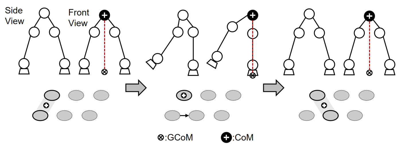
During the swing phase, the robot's torso shifts laterally to align the CoM with the GCoM, which is crucial to consider in the design of safe navigation algorithms for humanoid robots[4]. The calculation of the center of gravity involves the positions and masses of the supporting and swinging legs. Maintaining balance involves ensuring the gravity center stays within the support area. Deviations call for posture and joint torque adjustments, typically managed by PID controllers[5] or similar algorithms. This control strategy is advantageous as it prevents falls during the robot's walk by maintaining the center of gravity within the walking path. However, this safety can limit the robot's ability to walk without stoppage, potentially reducing dynamic walking efficiency.
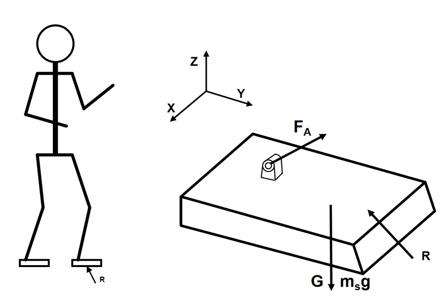
The following static balance equation of the foot can be derived: \begin{equation*} R + F_A + m_s g = 0 \end{equation*} \begin{equation*} OP \times R + M_A + OG \times m_s g + M_z + OA \times F_A = 0 \end{equation*}
2.3. Dynamic Walking (ZMP)
Dynamic walking is a widely used[6] and efficient strategy that allows bipedal robots to achieve speeds of less than one second per step. However, the inertia involved in this strategy makes it difficult for the robot to stop immediately, leading to instability during state transitions. To address this, the Zero Moment Point (ZMP)[7],[8] is introduced. During the single-leg support phase, ZMP is the projection of the robot's centre of gravity. When the ZMP is maintained within the support area, the robot remains stable and balanced. The ZMP is defined as the point where the horizontal components of the robot's main force, active moment, and torque equal zero on the ground, assuming sufficient friction between the robot's feet and the ground. In a one-foot support scenario, the leg exerts a force \(F_a\) and a moment \(M_a\) on the foot. The ground must apply a reaction force \(R\) and moments \(M_x, M_y, M_z\) at point \(P\) . By adjusting the position of \(P\) so that \(M_x\) and \(M_y\) become zero, the ZMP is achieved, ensuring the robot’s stability.
2.4. Linear Inverted Pendulum model
To design a feasible basic gait controller for a bipedal robot, the model of the biped robot can be simplified by assuming that the robot always has one foot on the ground. Consequently, the system can be modelled as a Linear Inverted Pendulum Model (LIPM). In this simplified model, the centre of mass of the bipedal system corresponds to the mass connected to the pendulum, and the ZMP on the landing foot corresponds to the position of the cart connected to the pendulum. The forward ZMP dynamic formula for one leg of the robot can be derived as follows: \begin{equation*} X_{zmp} = X_{mc} - \frac{l}{g} \dot{X}_{mc} \end{equation*} where \(X_{zmp}\) represents the forward Zero-Moment Point, \(X_{mc}\) represents the forward displacement of the center of mass, \(l\) is the length of the inverted pendulum, and \(g\) is the acceleration due to gravity.
2.5. Equation of motion of LIPM
[9] The inputs to the inverted pendulum system are the displacement of the cart and the expected tilt angle of the pendulum. The actual position signal of the cart and pendulum rod is collected in each sampling period and compared with the expected value. According to the comparison results, the corresponding control quantity is calculated by the control algorithm. In this system, one end of the pendulum is mounted on a cart so that the pendulum swings freely in a vertical plane. The cart moves horizontally along a fixed track. When no control is applied, the pendulum is in a stable equilibrium position, pointing straight up. In order for the pendulum to swing or maintain the stable upright position when there is force applied to the system, the cart needs to be controlled so that it is pulled forward or backward on the track.
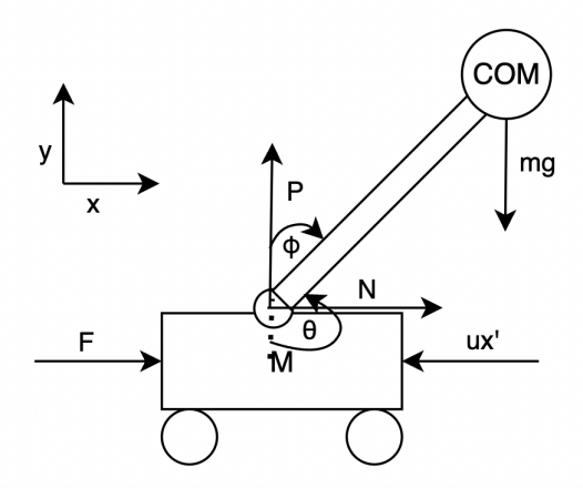
The force analysis of the system is based on Newton Classical mechanics. The following table shows the parameters used in formula derivation:
Table 1: Parameters of the system
| Parameter name | Meaning | Assumed value |
|---|---|---|
| \( M \) | Mass of cart | \( 1 \, kg \) |
| \( m \) | Mass of COM | \( 0.3 \, kg \) |
| \( u \) | Coefficient of friction | \( 0.02 \, kg\,m^{-2} \) |
| \( F \) | External force applied to cart | |
| \( x \) | Position of cart | |
| \( \theta \) | Swing angle of pendulum | |
| \( l \) | Distance of COM to the fulcrum | \( 0.3 \, m \) |
| \( I \) | Moment of inertia of pendulum | \( 0.5 \, N\,s^2/m \) |
| \( \phi \) | Angle between pendulum and vertical up |
The following equation can be obtained by analyzing the resultant force received in the horizontal direction of the cart:
The following equation can be obtained by horizontal pendulum force analysis:
Substitute equation ([???]) into ([???]) to obtain the first dynamic equation of the system:
Next, the resultant force in the vertical direction of the pendulum is analysed, which can be obtained: \begin{equation*} P = m \frac{d^2}{dt^2} (l\cos\theta) + mg \end{equation*} Rearrange: \begin{equation*} P = -ml\ddot{\theta}\sin\theta - ml\dot{\theta}^2\cos\theta + mg \end{equation*} Therefore, the moment equilibrium equation is: The moment equilibrium equation is given by:
The goal of the controller is to maintain the pendulum at an upright equilibrium position. Let \(\phi = \theta - \pi\) (the angle between the vertical upright position and the pendulum). Since \(\cos \phi = -\cos \theta\) , \(\sin \phi = -\sin \theta\) . Linearize at operating point \(\phi \approx 0\) : \(\sin \phi = -\phi\) , \(\cos \phi = -1\) , \(\ddot{\theta}^2 = 0\) . Combine and simplify equation ([???]) and ([???]) to obtain the linear dynamic functions of the system:
(I + m l^2) \ddot{\phi} - m g l \phi \&= m l \ddot{x} \end{align}
3. STATE FEEDBACK CONTROLLER DESIGN
In this section, the design and analysis of controllers of the LIPM model is introduced.
3.1. State space model of the system
From equation ([???]) and ([???]), derive the expression of \(\ddot{x}\) and \(\ddot{}ot{\phi}\) :
The state space expression:
\dot{y} \&= Cx \end{aligned} \end{equation}
The state vector \(x = [x, \dot{x}, \phi, \dot{\phi}]^T\) which are the position of the cart, the velocity of the cart, swing angle of the pendulum, the angular velocity of pendulum respectively. \(F\) is the control input. In order to write out the \(A\) matrix, the important elements are expressions of \(\dot{x}\) and \(\dot{\phi}\) in equation ([???]): \begin{equation*} \dot{x} = \frac{-u(I + ml^2)}{(I + ml^2)(M + m) - m^2l^2} \end{equation*} \begin{equation*} \dot{\phi} = \frac{-u(I + ml^2)}{(I + ml^2)(M + m) - m^2l^2} \end{equation*} Notice that the denominator of both expressions is the same constant, denote as \( c = (I + ml^2)(M + m) - m^2l^2 \) . Apply the similar procedure to \(\dot{\phi}\) , the \(A\) matrix can be obtained as:
0 \& \frac{-u(I + ml^2)}{c} \& \frac{m^2gl^2}{c} \& 0
0 \& 0 \& 0 \& 1
0 \& \frac{-uml}{c} \& \frac{(M + m) mgl}{c} \& 0 \end{bmatrix} \end{equation}
Similarly, extract the \(B\) matrix from equation ([???]) and ([???]):
\frac{I + ml^2}{c}
0
\frac{ml}{c} \end{bmatrix} \end{equation}
Consider the system outputs to be the same as the states, thus \(C\) matrix would be an identical matrix and \(D\) matrix would be a zero matrix:
0 \& 0 \& 1 \& 0 \end{bmatrix} \end{equation}
The system has two transfer functions because there are two outputs, the position of the cart ( \(x\) ) and the Angle of the pendulum ( \(\phi\) ), which can be affected by the input force ( \(F\) ):
The corresponding transfer functions can be calculated using ctrl from control library of Python.
3.2. Stability analysis
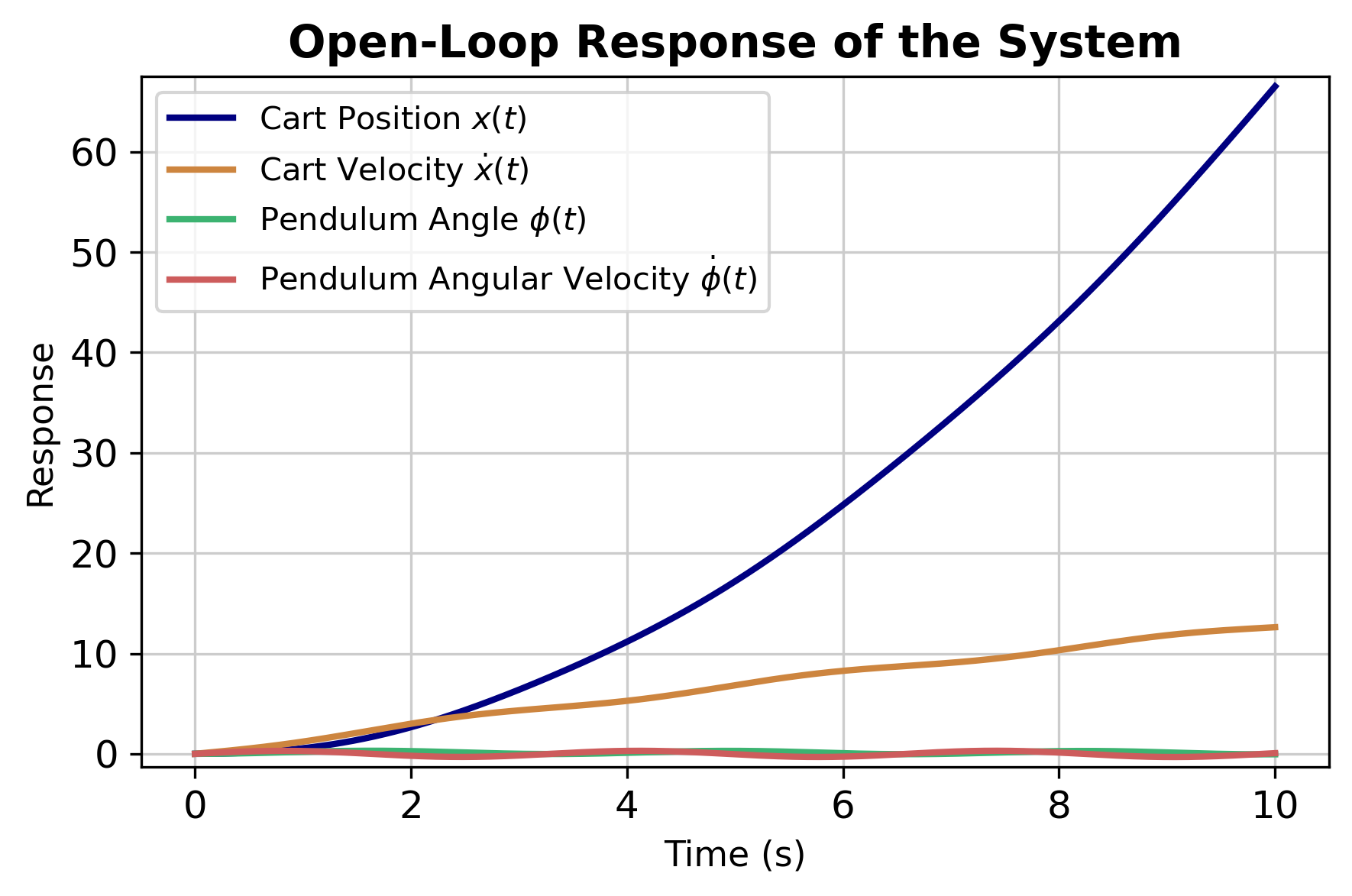
If the system deviates from the original equilibrium state due to the disturbance, but after the disturbance is removed, if it can be restored to the original equilibrium state, the system is said to be stable, otherwise the system is unstable. The easiest way to solve the stability problem of a linear system is to find all poles of the system and observe if there are any poles with real parts greater than zero (unstable poles). If there are such poles, the system is unstable, otherwise it is stable. The poles of \(G(s)x\) are: \(0, -0.077, 4.344, -4.361\) , and the poles of \(G(s)\phi\) are: \(-0.077, 4.344, -4.36\) . Both transfer functions have poles landed on the right half plane, therefore the system is unstable under open loop condition. Figure 4 shows the unstable response of the open loop system.
3.3. State feedback control
Adding a state feedback control to the system \( F = -Kx \) for some matrix \( K \) , now the closed-loop system becomes:
First, the system is required to have full rank in order to be controllable:
The \( n \times n \) controllability matrix:
0.61 \& -0.042 \& 1.556 \& -0.202
0 \& 1.027 \& -0.067 \& 13.466
1.027 \& -0.067 \& 13.466 \& -1.036 \end{bmatrix} \end{equation}
The Matrix has a rank of 4, therefore the system is controllable. In summary, the system is unstable but controllable. Thus, pole placement can be applied to move all the poles to the left-hand side plane to stabilize the system. The characteristic polynomial is then calculated:
\&= s^4 + a_1s^3 + a_2s^2 + a_3s + a_4 \end{aligned} \end{equation}
Put in reachable canonical form \(\dot{z} = \tilde{A}z + \tilde{B}u\) :
1 \& 0 \& 0 \& 1
0 \& 1 \& 0 \& 0
0 \& 0 \& 1 \& 0 \end{bmatrix}, \& \tilde{B} \&= \begin{bmatrix} 1
0
0
0 \end{bmatrix} \end{align}
The poles need to be designed so that the cart pendulum system can reach equilibrium without large oscillation. Therefore, the overshoot is designed to be 5%, damping ratio \(\zeta = 0.5\) , settling time \(t_s = 5\) , and natural frequency \(\omega_n = \frac{3.92}{t_s}\) . Two dominant poles are based on the choice of \(\zeta\) and \(\omega_n\) , the other two less dominant poles are placed 3 and 4 times further on the left plane which is set to be \(3\zeta\omega_n\) , \(4\omega_n\) . The expression of the desired characteristic polynomial is obtained:
where the poles are \(p_1 = 3.528\) , \(p_2 = 3.541\) , \(p_3 = 2.306\) , \(p_4 = 0.578\) . The state feedback matrix \(K\) is obtained:
Case 1:
Test the performance of state feedback controller with a step response. This step response makes the pendulum out of equilibrium.
Figure [???] shows the system quickly stabilizes the cart position in around 2 seconds while the pendulum angle reaches and maintains equilibrium rapidly, demonstrating effective state feedback control.
\bigskip
Case 2:
This case adds a step disturbance of \(5 \, N\) starting at \(t = 0\) . Initial condition of \(\phi = 0\) , \(x = 0\) . Such disturbance can be used to simulate a sudden and consistent effect on the system during operation thus test the adjustment ability of the system.
Figure [???] indicates a more volatile response to a 5N disturbance with higher peaks in cart displacement. Unlike the previous stable response, the cart and pendulum experience greater oscillations before stabilizing, showing robustness but with a more pronounced transient behaviour.
However, the cart position did not travel back to the initial position, this outlines the limitation of state feedback control, there is often an error which is usually removed by more advanced control strategies like PID control[10]. In the second half of the research, a Neural network controller will be implemented to remove the error and achieve better control outcomes.
4. NEURAL NETWORK CONTROLLER DESIGN
The integration of a neural network controller offers a sophisticated approach to managing nonlinear and complex systems like inverted pendulums[11]. Its ability to learn and adapt from data enables the controller to anticipate and compensate for uncertainties and variances in system dynamics, which traditional controllers might not handle efficiently. This adaptability and learning capability make neural networks particularly advantageous for enhancing system robustness and achieving superior performance in dynamic environments.
4.1. Generate training datas
The data set encapsulates the dynamic responses of an inverted pendulum system under various initial conditions and control inputs. It stimulates the pendulum's behaviour over time using a state-space model with random initial states, including small initial pendulum angles. The data set consists of states, control actions, and subsequent states, crucial for training a neural network to learn the system's complex dynamics and generalize well in different control scenarios. Experimental data gathering employed two methods: an uncontrolled state-space model for raw behaviour data and a refined state-space model with state feedback control for precise data. This dual approach explores the neural network model's data requirements.
4.2. Neural network
A feed-forward neural network was designed using PyTorch to model the control of an inverted pendulum system. The network accepts a four-dimensional input representing the system's state and processes it through two hidden layers, each containing 64 neurons and employing ReLU activation functions to introduce non-linearity. The output layer generates a single value, corresponding to the control force to be applied. The forward pass through the network can be described as:
where \(W_i\) and \(b_i\) are the weights and biases of the \(i\) -th layer, respectively. This architecture is intended to train on a dataset capturing the dynamics of the inverted pendulum, enabling the network to map system states to appropriate control actions, thereby maintaining stability.
4.3. Training the model
A process was established to train a neural network for controlling an inverted pendulum system. Pre-processed data, including system states and corresponding control forces, are loaded into PyTorch tensors. A neural network instance is initialized and trained using the Adam optimizer and mean squared error loss function, both standard choices for regression tasks. The loss function is defined as:
where \(y_i\) is the true force and \(\hat{y_i}\) is the predicted force. Over custom epochs, the network iteratively performs forward propagation to predict forces, calculates the loss, and updates the weights through back-propagation. The weight update rule for the Adam optimizer can be simplified as:
where \(\eta\) is the learning rate, and \(\hat{m_t}\) and \(\hat{v_t}\) are bias-corrected estimates of the first and second moments of the gradients. This methodology ensures the network learns to map system states to effective control actions for maintaining stability.
4.4. Performance of the Neural Network Controller using model trained with data from an uncontrolled state space model
First, generating training data for an inverted pendulum system by simulating 1000 samples. For each sample, a random initial state is created with the pendulum starting from a tilted position. A random force, ranging from -10 to 10 N, is applied to the system, and the resulting next state is calculated after a time step of 0.05 seconds. The initial states applied forces, and next states are saved for future neural network training.
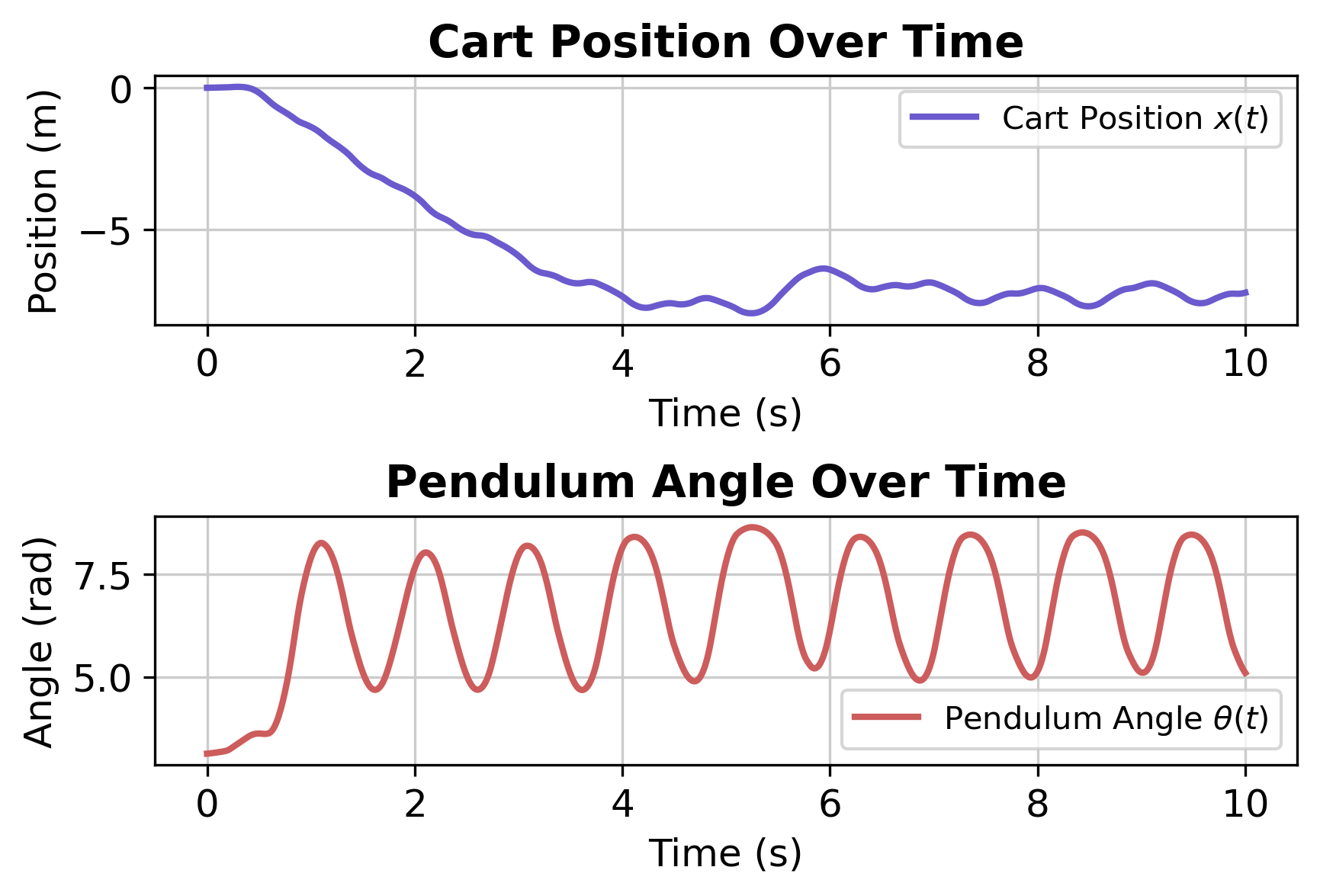
Based on the results shown in Figure5, the performance of the neural network controller is clearly sub-optimal. The cart position continuously deviates from the origin, exhibiting an unstable downward trend; meanwhile, the pendulum angle experiences large periodic oscillations and fails to reach a balanced state. This poor control outcome is primarily due to the use of untrained data for the control system. The untrained data fails to accurately capture the dynamic characteristics and control requirements of the system, leading to the neural network being unable to learn an effective control strategy, and ultimately, it fails to achieve stable control objectives. The High loss of the trained model also proves the point:
Epoch [1/1000], Loss: 32.6771125793457
...
Epoch [121/1000], Loss: 31.44316864013672
...
Epoch [991/1000], Loss: 18.984155654907227
4.5. Performance of the Neural Network Controller using model trained with data from a state space model with state feedback control
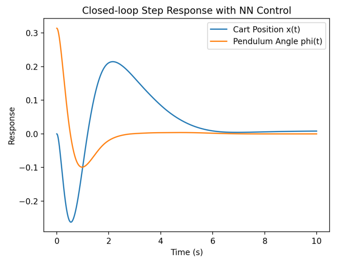
Case 1: 1000 epochs, 0.05 step length, 1000 sample. Using state space model with state feedback control. The pendulum is initially started from a tilted position and started with 5N external force.
Epoch [1/1000], Loss: 280.9759521484375
...
Epoch [121/1000], Loss: 57.45454406738281
...
Epoch [991/1000], Loss: 0.02957174740731716
In comparison to before, here, 1000 epochs can bring the loss down to a very low level. Figure 6 show stable control of both the cart and pendulum. Both cart and pendulum are stable around the 0 position which shows better system performance in comparison to the state feedback control.
Case 2: 1000 epochs, 0.05 step length, 1000 sample. Using state space model with state feedback control. The pendulum is initially started from a tilted position and started with 5N external force and add random (from -5 to 5N) disturbance during the process. From Figure [???], it can be seen that this controller exhibits strong robustness, achieving excellent control even in the presence of random disturbances.
4.6. Comparison of the two models
In the discussion of training outcomes, it was observed that datasets generated from an uncontrolled state space model resulted in higher loss post-training, leading to suboptimal control performance. Conversely, datasets derived from the refined state space model, which more accurately represent the system's dynamics, produced a significantly lower loss when used for training. The improved precision of the refined dataset evidently enhanced the neural network's ability to learn effective control strategies, as evidenced by its superior control capabilities. This underscores the importance of precise and representative training data in developing robust neural network controllers for complex dynamic systems.
5. Conclusion
In conclusion, the research presented here thoroughly demonstrates the effectiveness of a neural network controller in managing the dynamic challenges of an inverted pendulum system. The initial state feedback control method, while effective in certain scenarios, showed limitations in handling complex system dynamics. The subsequent integration of a neural network controller significantly enhanced control performance, as evidenced by lower loss metrics and improved response to disturbances. These findings underscore the potential of neural network controllers in advanced robotic and control systems, offering substantial improvements in adaptability and precision over traditional methods.
References
[1]. Hai-Wu Lee et al. “Research on the Stability of Biped Robot Walking on Different Road Surfaces”. In: ICKII. 2018, pp. 54–57. DOI: 10.1109/ICKII.2018.8569084.
[2]. S. H. Collins and A. Ruina. “A Bipedal Walking Robot with Efficient and Human-Like Gait”. In: Proceedings of the 2005 IEEE International Conference on Robotics and Automation. Barcelona, Spain, 2005, pp. 1983–1988. DOI: 10.1109/ROBOT.2005.1570404.
[3]. T. Sugihara, Y. Nakamura, and H. Inoue. “Real-time humanoid motion generation through ZMP manipulation based on inverted pendulum control”. In: Proceedings 2002 IEEE International Conference on Robotics and Automation. Vol. 2. Washington, DC, USA, 2002, pp. 1404–1409. DOI: 10.1109/ROBOT.2002.1014740.
[4]. Hanafiah Yussof and Masahiro Ohka. “Optimum Biped Trajectory Planning for Humanoid Robot Navigation in Unseen Environment”. In: (2010). DOI: 10.5772/9262.
[5]. Kiam Heong Ang, G. Chong, and Yun Li. “PID control system analysis, design, and technology”. In: IEEE Transactions on Control Systems Technology 13.4 (2005), pp. 559–576. DOI: 10.1109/ TCST.2005.847331.
[6]. Y. Okumura et al. “Realtime ZMP compensation for biped walking robot using adaptive inertia force control”. In: Proceedings 2003 IEEE/RSJ International Conference on Intelligent Robots and Systems (IROS 2003). Vol. 1. Las Vegas, NV, USA, 2003, pp. 335–339. DOI: 10.1109/ IROS.2003.1250650.
[7]. S. Kajita et al. “Biped walking pattern generation by using preview control of zero-moment point”. In: 2003 IEEE International Conference on Robotics and Automation. Vol. 2. Taipei, Taiwan, 2003, pp. 1620–1626. DOI: 10.1109/ROBOT.2003.1241826.
[8]. Miomir Vukobratovic and Branislav Borovac. “Zero-Moment Point - Thirty Five Years of its Life”. In: I. J. Humanoid Robotics 1 (2004), pp. 157–173. DOI: 10.1142/S0219843604000083.
[9]. M. W. Spong. Inverted Pendulum: Simulink Modeling. Control Tutorials for MATLAB and Simulink, University of Michigan. 2008. URL: https://ctms.engin.umich.edu/ CTMS/index.php?example=InvertedPendulum§ion=SimulinkModeling.
[10]. L. B. Prasad, B. Tyagi, and H. O. Gupta. “Optimal control of nonlinear inverted pendulum dynamical system with disturbance input using PID controller & LQR”. In: 2011 IEEE International Conference on Control System, Computing and Engineering. Penang, Malaysia, 2011, pp. 540–545. DOI: 10.1109/ICCSCE.2011.6190585.
[11]. David Rumelhart, Geoffrey Hinton, and Ronald Williams. “Learning representations by back- propagating errors”. In: Nature 323 (1986), pp. 533–536. URL: https://doi.org/10. 1038/323533a0.
Cite this article
Xie,Y.;Mi,Y. (2024). Optimizing inverted pendulum control: Integrating neural network adaptability. Applied and Computational Engineering,101,213-223.
Data availability
The datasets used and/or analyzed during the current study will be available from the authors upon reasonable request.
Disclaimer/Publisher's Note
The statements, opinions and data contained in all publications are solely those of the individual author(s) and contributor(s) and not of EWA Publishing and/or the editor(s). EWA Publishing and/or the editor(s) disclaim responsibility for any injury to people or property resulting from any ideas, methods, instructions or products referred to in the content.
About volume
Volume title: Proceedings of the 2nd International Conference on Machine Learning and Automation
© 2024 by the author(s). Licensee EWA Publishing, Oxford, UK. This article is an open access article distributed under the terms and
conditions of the Creative Commons Attribution (CC BY) license. Authors who
publish this series agree to the following terms:
1. Authors retain copyright and grant the series right of first publication with the work simultaneously licensed under a Creative Commons
Attribution License that allows others to share the work with an acknowledgment of the work's authorship and initial publication in this
series.
2. Authors are able to enter into separate, additional contractual arrangements for the non-exclusive distribution of the series's published
version of the work (e.g., post it to an institutional repository or publish it in a book), with an acknowledgment of its initial
publication in this series.
3. Authors are permitted and encouraged to post their work online (e.g., in institutional repositories or on their website) prior to and
during the submission process, as it can lead to productive exchanges, as well as earlier and greater citation of published work (See
Open access policy for details).
References
[1]. Hai-Wu Lee et al. “Research on the Stability of Biped Robot Walking on Different Road Surfaces”. In: ICKII. 2018, pp. 54–57. DOI: 10.1109/ICKII.2018.8569084.
[2]. S. H. Collins and A. Ruina. “A Bipedal Walking Robot with Efficient and Human-Like Gait”. In: Proceedings of the 2005 IEEE International Conference on Robotics and Automation. Barcelona, Spain, 2005, pp. 1983–1988. DOI: 10.1109/ROBOT.2005.1570404.
[3]. T. Sugihara, Y. Nakamura, and H. Inoue. “Real-time humanoid motion generation through ZMP manipulation based on inverted pendulum control”. In: Proceedings 2002 IEEE International Conference on Robotics and Automation. Vol. 2. Washington, DC, USA, 2002, pp. 1404–1409. DOI: 10.1109/ROBOT.2002.1014740.
[4]. Hanafiah Yussof and Masahiro Ohka. “Optimum Biped Trajectory Planning for Humanoid Robot Navigation in Unseen Environment”. In: (2010). DOI: 10.5772/9262.
[5]. Kiam Heong Ang, G. Chong, and Yun Li. “PID control system analysis, design, and technology”. In: IEEE Transactions on Control Systems Technology 13.4 (2005), pp. 559–576. DOI: 10.1109/ TCST.2005.847331.
[6]. Y. Okumura et al. “Realtime ZMP compensation for biped walking robot using adaptive inertia force control”. In: Proceedings 2003 IEEE/RSJ International Conference on Intelligent Robots and Systems (IROS 2003). Vol. 1. Las Vegas, NV, USA, 2003, pp. 335–339. DOI: 10.1109/ IROS.2003.1250650.
[7]. S. Kajita et al. “Biped walking pattern generation by using preview control of zero-moment point”. In: 2003 IEEE International Conference on Robotics and Automation. Vol. 2. Taipei, Taiwan, 2003, pp. 1620–1626. DOI: 10.1109/ROBOT.2003.1241826.
[8]. Miomir Vukobratovic and Branislav Borovac. “Zero-Moment Point - Thirty Five Years of its Life”. In: I. J. Humanoid Robotics 1 (2004), pp. 157–173. DOI: 10.1142/S0219843604000083.
[9]. M. W. Spong. Inverted Pendulum: Simulink Modeling. Control Tutorials for MATLAB and Simulink, University of Michigan. 2008. URL: https://ctms.engin.umich.edu/ CTMS/index.php?example=InvertedPendulum§ion=SimulinkModeling.
[10]. L. B. Prasad, B. Tyagi, and H. O. Gupta. “Optimal control of nonlinear inverted pendulum dynamical system with disturbance input using PID controller & LQR”. In: 2011 IEEE International Conference on Control System, Computing and Engineering. Penang, Malaysia, 2011, pp. 540–545. DOI: 10.1109/ICCSCE.2011.6190585.
[11]. David Rumelhart, Geoffrey Hinton, and Ronald Williams. “Learning representations by back- propagating errors”. In: Nature 323 (1986), pp. 533–536. URL: https://doi.org/10. 1038/323533a0.