1. Introduction

PD, PI, and PID controls are fundamental and widely used in mechatronics and automated fields. As all textbooks say the proportional control is to process the input signal multiple times till it reaches 0 error. With higher gain, and the lower the error is. However, there are cases in which error is small but can’t be eliminated, the integral control is introduced. It is a “memory” component that accumulates the error from proportional control and return the feedback to the input. It can make the system stable with 0 error, but the initial overshoot appears. The derivative control controls the rate of change in error and gives a negative output to reduce the rate of change in order to mitigate the overshoot. These are the fundamental properties of the control under ideal conditions. That is also the premise of the transfer function and the impedance of each component is calculated. However, when assembled in reality, there are differences. One reason is that the passive components contain other properties. For example, the resistor may also have inductance and capacitance, but they are minimal compared to resistance. The impedance is also calculated based on that. In real life, these values. The other reason is that in theory, the input and output signal can be infinitely large, but the control mechanism is not. When saturated, the control can not process a larger signal than the designed maximum value, causing undesirable performances. Hence, it is important to prevent saturation when designing controllers. [1]

2. Saturation

Saturation is a term commonly used in multiple areas. For example, the current is saturated in a close-loop circuit with 0 resistance. In the field of nonlinear electrical controllers, the output of the controller can be infinitely large in theory, but the actuator will stop processing a higher signal compared to its saturation value. [2]

2.1. Saturation function

The saturation function is defined as that in its domain of definition, when the value chosen is out of the domain, the value of the function remains unchanged.[3] To be specific, the purpose of the saturation function is to restrict the range of viable values for simulating a physical system. In the case of controllers, it restricts the output signal in order to prevent saturation. The saturation function is generally expressed in hyperbolic tangent and sigmoid functions. The general expression of the saturation function sat(x) is defined as:

\( sat(x)\begin{cases} \begin{array}{c} c if f \gt c (1) \\ f if |f|≤c (2) \\ -c if f \lt c (3) \end{array} \end{cases} \)

Where f is a linear function and c is a positive constant.

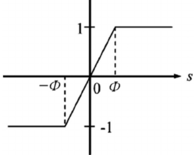
Figure 1. Graph of sigmoid function.

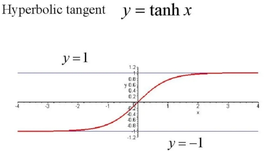
Figure 2. Graph of hyperbolic tangent function.

The graphs above have asymptotes at certain values, which constrain the value of input in a certain range and avoiding overloading the components.[4]

2.2. Implementing the saturation function

In the classical control laws[3], the PD, PI, and PID control are expressed as the following:

\( {τ_{PD}}={K_{P}}e(t)+{K_{D}}\frac{de(t)}{dt} \) \( (4) \)

\( {τ_{PI}}={K_{P}}e(t)+{K_{I}}\int _{0}^{t}e(s)ds \) \( (5) \)

\( {τ_{PID}}={K_{P}}e(t)+{K_{I}}\int _{0}^{t}e(s)ds{+K_{D}}\frac{de(t)}{dt} \) \( (6) \)

Where \( {K_{P}} \) , \( {K_{D}} \) , and \( {K_{I}} \) are the gain of each controller respectively.

This form of equations is best at designing linear controllers, but there are also other types of controllers such as nonlinear ones. In the case of nonlinear controllers, the tracking speed is significantly faster than the linear controllers, but the load on the electrical components are high, which can cause saturation. Therefore, the process of clamping is utilized to control the degree of saturation. To implement clamping, the control laws are expressed as the following:

\( {τ_{PD}}=sat[{K_{P}}e(t)]+sat[{K_{D}}\frac{de(t)}{dt} \) ](7)

\( {τ_{PI}}={sat[K_{P}}e(t)]+{sat[K_{I}}\int _{0}^{t}e(s)ds] \) (8)

\( {τ_{PiD}}=sat[{K_{P}}e(t)]+sat[{K_{I}}\int _{0}^{t}e(s)ds]{+sat[K_{D}}\frac{de(t)}{dt} \) ](9)

In this form, the saturation function is processed first to limit the received input from the source, and then, the signal is sent to the controllers. The saturation function is implemented before each controllers, providing a comprehensive prevention for saturation in each controller.

2.3. Root locus method and stability

The root locus method is an approach to analyze the stability of the controller expressed in the form of the transfer function. The transfer function is an expression that relates the linear input and output in a Laplace transformed ratio in a time invariant system, generally in a first order differential equation with the initial condition set to be 0.

The Lyapunov method is a more advanced version of the root locus method. It applies in both nonlinear and linear controllers, whereas the root locus method applies only in linear systems.[6]

The step response plot is a straightforward Heaviside step function of how the controller’s behavior based on the transfer function. It showed the time evolution in the output of the controller. [4]By checking the step response plot, tuning the controller until it has desirable performance and proper values for each electrical components is easier. It also provides valuable information to tune the system to prevent saturation.

The pzmap( pole-zero map) is a function in Matlab and Octave to indicate the poles and zeros respectively. In a continuous linear system, checking the zeros and poles is a direct way of detecting where the stable and unstable locus of the system are. A stable locus can minimize unstable fluctuations in order to prevent overload.[7]

3. Case analysis

Consider a fast-tracking Linear PD control of a DC motor, the input signal is a square wave of 50 mHz and a voltage of 10 mV. In order to track the reference signal with zero error in a short amount of time. The gain of the controller needs to be considerably high, and the gain of the proportional control in this design is chosen to be less than or equal to 10, in this example, the initial gain is 10. The transfer function of the system is G(s)=0.65s+10, the simulation is conducted on Octave.online. Figure 3 is the step response and Figure 4 is the root locus of the proposed PD controller.

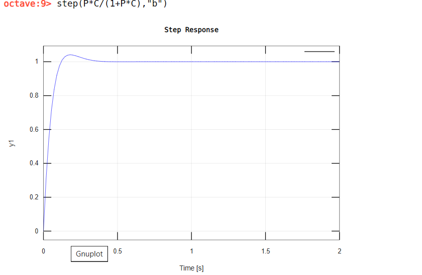
Figure 3. plot of step response for the designed controller.

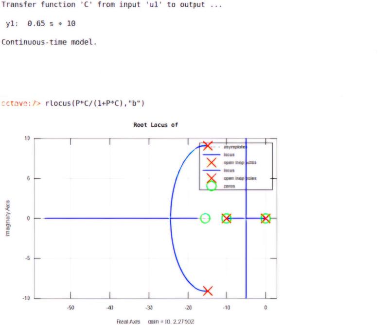
Figure 4. Root locus plot of the controllers.

The simulation showed a stable step response with a slight overshoot. The tracking of the reference signal is completed in less than 0.5 seconds, which is a good performance. The root locus and pzmap graph showed the stable points and poles of the transfer function. Based on the analysis, the controllers are built on Falstad.com.

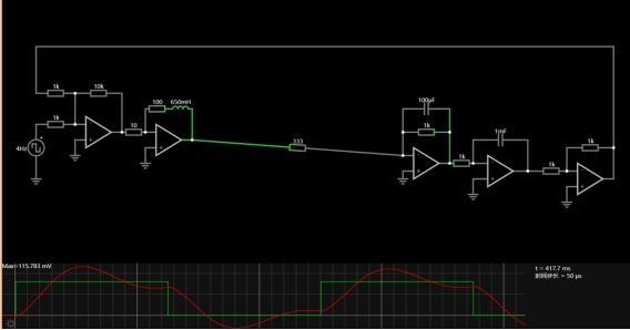
Figure 5. Figure of the built controllers.

In the built system, the step response is different than the simulation and is unstable. In this case, it is suspected that the system is saturated. The tuning process is conducted to change the transfer function and the value for electrical components. The image below is the system after tuning.

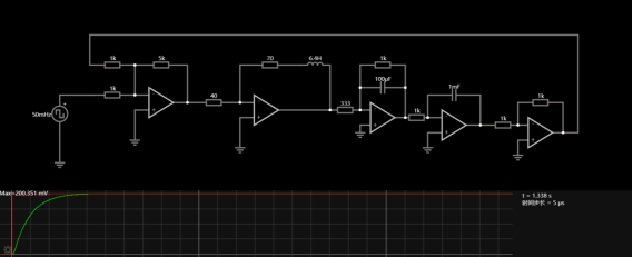
Figure 6. Figure of the tuned circuit.

The tuned system showed a fast and stable reference signal tracking with minimum overshoot. It can be concluded that the system is unsaturated and has good performance. Future improvements will be made to the value of the inductor. In the simulation, the inductance is 6.4H, which in reality is a large inductor. The controllers and the DC motor in the design are supposed to be small in size and the value for each components is small. Another improvement is to check if it can also capable of tracking other types of input signals with the same precision and characteristics as the square wave. In the future, the saw-tooth and triangular input will be tested on this system.

4. Discussion

The above analyses are all conducted in the ideal models and environments. In real life, there are multiple factors that can cause the discrepancies between simulations and experiments. One of them may be due to temperature changes. For example, in physics, TCR (temperature coefficient of resistance) describe a term describing the change in resistance with respect to temperature changes with a unit of ppm/K, parts per million per Kelvin. It sets an important parameter of that describes the performance of the resistor in detail. Other electrical components also have similar parameter. The definition of electrical load[8] is that as the system work, the system takes electrical input energy and transfers it to heat. It can be resistive, capacitive, inductive, and a combination of all. When the electrical load on certain components is high, it can cause an increase in temperature, which reduces the performance of components. The stability of the system can be deteriorated, causing saturation. It’s best to put a thermal detector on the system to control the temperature so that the system is working in perfect thermal condition.

The other one may due to the disregarded properties of electrical components[9]. In the calculation of impedance, the ideal model of components are applied in the calculation with ideal resistor dissipating electrical power to heat and ideal inductor turning electrical power to magnetic field. Resistor not only has resistance in practice, but also has inductance and capacitance, which are small comparing to resistance and often disregarded. However, depending on the application of electrical components, these properties can have significant impact on the system, especially in high frequency AC applications. The term parasitic inductance is accounted based on the discrepancies between ideal simulation and real practice. To prevent this from distorting the experiments and design, it’s best to check the detailed information sheets provided by the manufacturer of the electrical components[10].

5. Conclusion

The paper has investigated the saturation control in details with an example of a PD circuit. The saturation function is the most effective way to clamp the controller to avoid saturation which preventing the system from operating under normal conditions. By checking the value of non-clamping and clamping, it is clear to see how saturated the system is: if the values are the same, the system is unsaturated; if the two values are different, the system is saturated. The classical way of using root locus method and pz map is to find the stability of the controller, which contributes greatly in optimizing the performance of the system. Saturation can disturb the performance of the system, and even deteriorate the stability, making the system malfunction. The above methods are important in controller design and tuning. When designing the controllers, it is also crucial to consider the physical properties of electrical components since the environmental differences can have great impact on the performance of the entire system. Checking the detailed information provided by manufacturers and controlling the working conditions can mitigate the effects.

References

[1]. [1] Sun, Y., & Wang, L. (2013). On stability of a class of switched nonlinear systems. Automatica, 49(1), 305–307. https://doi.org/10.1016/j.automatica.2012.10.011
[2]. [2] Zhang, J., & Raissi, T. (2019). Saturation control of switched nonlinear systems. Nonlinear Analysis. Hybrid Systems, 32, 320–336. https://doi.org/10.1016/j.nahs.2019.01.005
[3]. [3] Guerrero, J., Torres, J., Creuze, V., Chemori, A., & Campos, E. (2019). Saturation based nonlinear PID control for underwater vehicles: Design, stability analysis and experiments. Mechatronics, 61, 96–105. https://doi.org/10.1016/j.mechatronics.2019.06.006
[4]. [4] Caverly, R. J., Zlotnik, D. E., Bridgeman, L. J., & Forbes, J. R. (2014). Saturated proportional derivative control of flexible-joint manipulators. Robotics and Computer-integrated Manufacturing, 30(6), 658–666. https://doi.org/10.1016/j.rcim.2014.06.001
[5]. [5] Palani, S. (2022). Root Locus Method for Analysis. In: Automatic Control Systems. Springer, Cham. https://doi.org/10.1007/978-3-030-93445-3_5
[6]. [6] Campos, E., Monroy, J., Abundis, H., Chemori, A., Creuze, V., & Torres, J. (2019). A nonlinear controller based on saturation functions with variable parameters to stabilize an AUV. International Journal of Naval Architecture and Ocean Engineering, 11(1), 211–224. https://doi.org/10.1016/j.ijnaoe.2018.04.002
[7]. [7] Pole-zero plot of dynamic system - MATLAB pzmap. (n.d.). https://www.mathworks.com/help/control/ref/lti.pzmap.html
[8]. [8] T, A. (2017, March 20). Electrical load. Circuit Globe. https://circuitglobe.com/electrical-load.html
[9]. [9] Williams, B. W. (1992). Power Electronics: devices, drivers, applications and passive components. http://ci.nii.ac.jp/ncid/BA1827230X
[10]. [10] R Goldstein - Vishay Foil Resistors, Tech. Note, 2018 - foilresistors.com
Cite this article
Duan,Y. (2024). Design and optimization of PD control system based on saturation. Applied and Computational Engineering,102,90-95.
Data availability
The datasets used and/or analyzed during the current study will be available from the authors upon reasonable request.
Disclaimer/Publisher's Note
The statements, opinions and data contained in all publications are solely those of the individual author(s) and contributor(s) and not of EWA Publishing and/or the editor(s). EWA Publishing and/or the editor(s) disclaim responsibility for any injury to people or property resulting from any ideas, methods, instructions or products referred to in the content.
About volume
Volume title: Proceedings of the 2nd International Conference on Machine Learning and Automation
© 2024 by the author(s). Licensee EWA Publishing, Oxford, UK. This article is an open access article distributed under the terms and
conditions of the Creative Commons Attribution (CC BY) license. Authors who
publish this series agree to the following terms:
1. Authors retain copyright and grant the series right of first publication with the work simultaneously licensed under a Creative Commons
Attribution License that allows others to share the work with an acknowledgment of the work's authorship and initial publication in this
series.
2. Authors are able to enter into separate, additional contractual arrangements for the non-exclusive distribution of the series's published
version of the work (e.g., post it to an institutional repository or publish it in a book), with an acknowledgment of its initial
publication in this series.
3. Authors are permitted and encouraged to post their work online (e.g., in institutional repositories or on their website) prior to and
during the submission process, as it can lead to productive exchanges, as well as earlier and greater citation of published work (See
Open access policy for details).