1. Introduction

Differential equations (DEs), particularly Partial Differential Equations (PDEs), are fundamental in modeling complex phenomena across various scientific disciplines, such as the Schrödinger equation. It describes the evolution of the quantum state of a system, and the nonlinear Black-Scholes equation, used to model derivative pricing under market impact. PDEs are crucial for describing systems with multiple variables and their interactions. However, finding analytical solutions is frequently infeasible because of their intrinsic complexity, non-linearity, and multi-dimensionality. Approximating PDE solutions is typically addressed through conventional numerical methods such as spectral methods, finite difference schemes, and finite element analysis [1]. Nonetheless, these approaches encounter significant obstacles, such as elevated processing expenses, limitations in handling intricate boundary conditions, and restricted scalability in high-dimensional problems.

Despite improvements in traditional methods, their limitations remain, particularly when dealing with complex boundary conditions, high-dimensional spaces, and real-time applications. The “curse of dimensionality” remains a significant obstacle, as computational costs increase exponentially with the number of dimensions [2]. Accuracy is also compromised in scenarios requiring fine resolution or fast processing times.

Over recent years, the advent of deep learning has introduced innovative approaches to addressing differential equations, with a particular emphasis on the application of neural networks [3]. Among these advancements, Convolutional Neural Networks (CNNs) have attracted considerable interest due to their proficiency in handling grid-like data, making them well-suited for problems involving spatial hierarchies [4]. Neural networks offer distinct advantages over traditional methods, including learning directly from data, adapting to complex and irregular domains, and generalizing across diverse problem settings [5]. These capabilities make them promising for tackling the challenges posed by PDEs.

This article highlights the application of neural networks for resolving differential equations, focusing on the innovations that have emerged in recent years. The existing work is categorized into three main approaches: data-driven, physics-driven, and hybrid-driven methods. Data-driven methodologies employ extensive datasets to train neural networks, with the goal of establishing immediate correlations between inputs and solutions. Physics-driven methods exploit the underlying physical laws for the model training, which ensures the solutions are consistent with the governing equations. Hybrid-driven methods combine the strengths of both approaches, using data to inform the network while enforcing physical constraints. By examining these methods, this paper provides a comprehensive overview of current research, evaluates strengths and limitations, and suggests directions for future work.

2. Deep learning methods for solving DEs

The application of neural network to solve differential equations represents a significant shift in how these mathematical problems are approached.

Traditionally, solving PDEs like the ones represented by the general form:

\( F(x,u(x),∇u(x),{∇^{2}}u(x), λ)=0, x∈Ω \) (1)

\( B(u,x)=0, x∈∂Ω \) (2)

, where \( x∈[{x_{1}}, …,{ x_{n}}{]^{T}}∈Ω \) , and \( Ω⊂{R^{n}} \) represents the domain; \( u(x) \) is the unknown solution; \( ∇ \) is the differential operator; \( λ \) is parameters; \( B(u,x) \) gives the boundary conditions.

The solution of the equation could be given by the combination of parameters \( λ \) and \( u(x) \) which satisfies Eq.1 and Eq.2. It could be assumed that the \( u(x) \) can be approximated by a neural network \( \hat{u}(x;W,b) \) , where \( W \) denotes the weight matrices and \( b \) denotes the bias in the neural network. The neural network’s output, which approximates the solution \( u(x) \) , is given by:

\( \hat{u}(x;W,b)=σ({W^{(L)}}σ({W^{(L-1)}}…σ({W^{(1)}}x+{b^{1}})…+{b^{(L-1)}})+{b^{(L)}}) \) (3)

, where \( σ \) is the activation function (e.g., ReLU, sigmoid), and \( L \) is the number of layers in the neural network.

To ensure that the neural network's predictions align with the PDE and its boundary conditions, a mean squared error (MSE) loss function will be crafted as part of the training regimen. Usually, the PDE and the boundary condition are represented by two terms in the loss function:

\( L(W,b)={L_{PDE}}+{L_{BC}} \) (4)

The PDE loss \( {L_{PDE}} \) ensures that the network output satisfies the PDE:

\( {L_{PDE}}=\frac{1}{N}\sum _{i=1}^{N}||F({x_{i}},{\hat{u}_{i}}({x_{i}};W,b),∇\hat{u}({x_{i}};W,b),{∇^{2}}\hat{u}({x_{i}};W,b),λ) {||^{2}} \) (5)

, where \( {x_{i}} \) are points sampled from the domain \( Ω \) .

The boundary condition loss \( {L_{BC}} \) verifies that the network's output satisfies the boundary conditions.:

\( {L_{BC}}=\frac{1}{M}\sum _{j=1}^{M}||B(\hat{u}({x_{j}};W,b),{x_{j}}) {||^{2}} \) (6)

, where \( {x_{j}} \) are points sampled from the boundary \( ∂Ω \) .

In actual use, the formula of the loss function can also be appropriately adjusted based on the information obtained from the initial data.

2.1. Data-driven methods

Data-driven approaches to solving differential equations involve directly applying large datasets to train neural networks. These datasets usually consist of input-output pairs, where the input includes information such as initial or boundary values, and the output is the corresponding solution to the differential equation. This methodology does not directly integrate the intrinsic physical laws to the system, but rather relies solely on the network’s ability to learn the mapping between inputs and solutions from data.

2.1.1. Training data generation. In many cases, the training data for data-driven methods is generated synthetically using traditional numerical methods. For a given particular PDE, numerical solvers like finite difference methods can be employed to produce solutions corresponding to different initial and boundary conditions. Noise can be added to these solutions to enhance the model’s robustness and generalization [6]. These synthetic datasets serve as the “ground truth” for training the model. The dataset typically consists of pairs where \( {x_{i}} \) , \( {u_{i}} \) , where \( {x_{i}} \) represents the input conditions (such as spatial coordinates or initial values), and \( {u_{i}} \) represents the corresponding solution values. The model is then trained for minimizing the error between its predictions and these known solutions.

2.1.2. Neural network architecture. During solving differential equations, neural network architectures can be designed to handle either continuous- or discrete-time models [7]. The choice between these two approaches depends on the problem 's characteristics, the data available, and the desired outcome.

2.1.3. Continuous-time models. This model represents the system’s dynamics as a function of continuous variables, such as space and time. In these models, differential equations are defined over a continuous domain, and the solution is typically sought as a continuous function.

In continuous-time models, the neural network is designed to approximate a continuous function that satisfies the differential equation across the entire domain. The network typically takes continuous input variables (e.g., time \( t \) and spatial coordinates \( x \) ) and outputs the predicted solution \( u(t,x) \) . For instance, a feedforward network in a continuous-time model might take the following form:

\( \hat{u}(t,x;W,b)={σ_{3}}[{W^{{(3)^{T}}}}{σ_{2}}[{W^{{(2)^{T}}}}{σ_{1}}[{W^{{(1)^{T}}}}(\frac{t}{x})+{b^{(1)}}]+{b^{(2)}}]+{b^{(3)}}] \) (7)

The network outputs the continuous function \( \hat{u}(t,x) \) , which approximates the solution to the differential equation.

2.1.4. Discrete-time models. Discrete-time models represent the system’s behavior at specific time steps. The differential equations are discretized, and the solution is computed at discrete intervals. This approach is often used when the system evolves over time in distinct steps, or when data is available only at certain time points.

In discrete-time models, is engineered to predict the system's state at the subsequent time step, based on its current state. This type of architecture often involves recurrent neural networks (RNNs) or other temporal models that can capture the dynamics over time. For example, in a discrete-time setting, a feedforward network might take the form:

\( {\hat{u}_{n+1}}={σ_{2}}[{W^{{(2)^{T}}}}{σ_{1}}[{W^{{(1)^{T}}}}{\hat{u}_{n}}+{b^{(1)}}]+{b^{(2)}}] \) (8)

, where \( {\hat{u}_{n}} \) represents the system’s state at the current step n; \( {\hat{u}_{n+1}} \) is the network predicts for the state at the n + 1 step.

2.2. Physics-driven methods

Physics-Informed Neural Networks (PINNs) have become a potent instrument in the field of physics-based differential equation solving techniques. [8]. Unlike traditional approaches that require extensive data or purely numerical solutions, PINNs incorporate the physical rules during training procedure directly.

PINNs can solve forward problems, which means it can predict the future state of a system given initial and boundary conditions, and inverse problems, where the aim is to infer unknown parameters or functions within the PDEs [9].

2.2.1. Introduction of PINN. PINN leverages models to estimate the PDEs’ solution while simultaneously satisfying the physical constraints of the equations. The structure of a PINN integrates both the data and the physics into the learning process. As shown in Figure 1, the key components of PINN include the neural network architecture, different loss components (data, PDE, boundary conditions, and initial conditions), and the overall loss.

2.2.2. Neural network architecture. In a typical PINN, the model is designed to take the spatial coordinates \( x \) and time \( t \) as inputs and produce the corresponding solution \( \hat{u}(t,x) \) as output, as demonstrated in Figure 1. The network’s output \( \hat{u} \) is then utilized to determine the various loss function components that direct the network's training. The model is made up of multiple layers, with each layer applying both linear and nonlinear activation functions. The network’s architecture can vary in depth and width depending on the complexity of the problem.

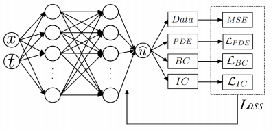
Figure 1. Representative structure of a feedforward neural network for PINN (Figure Credits: Original).

There are four losses: (1) Data Loss \( {L_{data}} \) : This term represents the MSE between the network’s predictions and any available observational or experimental data. It ensures the output of network aligns with known data points. (2) PDE Loss \( {L_{PDE}} \) : This term enforces the governing PDE across the domain. It is computed by evaluating the residuals of the PDE at a set of collocation points. The network is trained to minimize these residuals, thereby ensuring that the solution satisfies the PDE. (3) Boundary Condition Loss \( {L_{BC}} \) : This term guarantees that the network's output conforms to the boundary conditions. It penalizes deviations from the boundary conditions at the boundary points. (4) Initial Condition Loss \( {L_{IC}} \) : For time-dependent problems, this component ensures that the network's forecasts are in accordance with the initial conditions at the simulation's commencement.

2.2.3. Training process. The ability of PINNs to compute the required derivatives for the PDE residuals through automatic differentiation is one of its main advantages. This technique allows the model to efficiently calculate gradients with respect to the input variables, which are crucial for minimizing the PDE loss.

The training involves optimizing the neural network’s parameters to minimize the total loss \( L \) . This is typically done using gradient descent-based optimization algorithms, such as the Adam optimizer. To guarantee the anticipated solution fulfills the data, PDE, boundary conditions, and initial conditions, the network modifies its parameters throughout training in order to minimize the loss.

2.3. Hybrid-driven methods

These methods represent a synergistic model that unifies the advantages of both data-driven and physics-driven (specifically, PINN-based) methodologies. These methods aim to leverage the power of data where it is abundant and reliable while ensuring that the solutions respect the underlying physical laws of the system. In many practical scenarios, there is a mixture of available data and known physical laws, but neither alone is sufficient to produce a robust solution. Hybrid-driven methods address this by blending the two approaches, ensuring that the neural network solutions are both accurate with respect to data and consistent with physical principles.

2.3.1. Network architecture. In hybrid-driven methods, the neural network architecture can be designed to accommodate both data-driven and physics-driven components. One common approach is to have a single neural network that outputs the solution \( \hat{u}(t,x) \) , which is then subject to both a data- and physics-based loss.

Alternatively, the architecture might involve separate subnetworks—one for modeling the data-driven aspects and another for enforcing the physics. These subnetworks could then be combined at a later stage in the architecture to produce the final solution

2.3.2. Training process. The loss function in hybrid-driven methods typically combines both data- and physics-driven terms. The loss function can be normally described as:

\( L(W,b)={αL_{data}}+β{L_{PDE}}+γ{L_{BC}}+δ{L_{IC}} \) (9)

, where \( {L_{data}} \) , \( {L_{PDE}} \) , \( {L_{BC}} \) and \( {L_{IC}} \) are mentioned before in Section 2.2.2. For parameters \( α,β,γ,δ \) they are weighting factors that balance the contributions of the different loss components. These weights can be adjusted based on the relative confidence in the data versus the physical model, or they can be learned as part of the training process.

Another implementation strategy is to use physics-based simulations to augment the training data. When empirical data is limited, simulations based on known physics can generate additional data points, which the neural network can use for training. This augmented data helps improve the network’s performance and ensures that the derived solution aligns with the principles of physics.

3. Discussion

The application of solving differential equations leveraging neural networks marks a significant advancement in both numerical analysis and machine learning. Each of the approaches discussed—data-driven methods, physics-driven methods (with a focus on PINNs), and hybrid-driven methods—offers distinct advantages and presents unique challenges.

3.1. Data-driven methods

These methods perform very well when there is enough high-quality data available to begin with. These methods allow neural networks to learn complex mappings directly from the data, often achieving high accuracy in the domain covered by the training data. As Berg and Nyström demonstrate, high-quality data allows data-driven methods to accurately discover and model complex physical processes using neural networks [10]. Their work illustrates that with the right data and model selection, even com- plex PDEs can be effectively reverse-engineered, leading to highly accurate simulations. However, data-driven methods face significant challenges when extrapolating beyond the training set because they do not enforce the laws of physics themselves. Rudy et al. highlight a significant limitation of data-driven neural networks in the presence of noise [11]. They demonstrate that while neural networks can accurately identify the correct terms in a complex PDE like the Kuramoto-Sivashinsky equation, noise introduces substantial errors in the coefficients. This underlines the sensitivity of data-driven methods to noise, which can lead to significant inaccuracies in the learned models, especially when numerical differentiation is involved.

3.2. PINNs

PINNs directly include physical laws during training, hence addressing some of the main drawbacks of data-driven techniques. PINNs guarantee that the solutions comply with the underlying physics by minimizing the residuals of the PDEs, boundary conditions, and beginning conditions. This makes them particularly powerful in scenarios where data is limited or when it is crucial to maintain physical consistency [12]. However, PINNs can be computationally expensive and may encounter difficulties with optimization due to the complex loss landscapes they generate [13].

3.3. Hybrid-driven methods

Hybrid methods strike a balance, leveraging the advantages of both data- and physics-driven strategies. By integrating data with physical constraints, these methods can achieve high accuracy while ensuring that the solutions respect the underlying physical laws. Hybrid methods are especially useful in real-world applications where both data and physics are available but neither alone is sufficient. The main challenges with hybrid methods include the complexity of designing and training the models, as well as the need to balance the contributions of data-driven and physics-driven components in the loss function.

4. Conclusion

Neural networks have introduced a transformative approach to solving differential equations, offering methods that synergize traditional numerical techniques with advanced machine learning capabilities. This study examined three primary approaches: data-driven methods, physics-driven methods (specifically Physics-Informed Neural Networks, or PINNs), and hybrid- driven methods. Data-driven methods are highly effective in scenarios where extensive datasets are available, llowing neural networks to acquire intricate relationships from the data. However, these methods often face challenges in generalization and may produce solutions that lack physical consistency when applied beyond the scope of the training data. Physics-driven techniques, especially PINNs, overcome constraints by incorporating the fundamental physical laws directly into the neural network's loss. This merging guarantees that the solutions produced by the network are not just consistent with the data but also comply with the foundational physical principles. While PINNs are particularly well-suited for problems with sparse data or where physical accuracy is paramount, they are often computationally intensive and can be challenging to optimize due to the complexity of the loss landscape. Hybrid-driven methods represent a convergence of data- and physics-driven approaches, exploiting both their strengths. By combining empirical data with physical constraints, these methods achieve enhanced accuracy and generalization, making them especially suitable for complex real-world applications where both data and physics are integral.

Future research directions are likely to focus on improving the scalability and efficiency of these methods, integrating them with traditional numerical approaches, and incorporating uncertainty quantification. Additionally, extending these methodologies to emerging interdisciplinary domains and enhancing the interpretability of neural network models will be critical for their broader adoption.

In conclusion, neural networks provide a robust and versatile framework for solving differential equations, with each approach—data-driven, physics- driven, and hybrid-driven—offering distinct advantages. It is anticipated that these approaches will become more and more important as they advance in solving challenging problems in a variety of technical domains.

References

[1]. Ames, W. F. (2014). Numerical methods for partial differential equations. Academic press.
[2]. Bellman, R., & Kalaba, R. (1957). Dynamic programming and statistical communication theory. Proceedings of the National Academy of Sciences, 43(8), 749-751.
[3]. Beck, C., Hutzenthaler, M., Jentzen, A., & Kuckuck, B. (2020). An overview on deep learning-based approximation methods for partial differential equations. arXiv preprint arXiv:2012.12348.
[4]. Lee, S., Kim, H., Lieu, Q. X., & Lee, J. (2020). CNN-based image recognition for topology optimization. Knowledge-Based Systems, 198, 105887.
[5]. Blechschmidt, J., & Ernst, O. G. (2021). Three ways to solve partial differential equations with neural networks—A review. GAMM‐Mitteilungen, 44(2), e202100006.
[6]. Maslyaev, M., Hvatov, A., & Kalyuzhnaya, A. (2020). Data-driven partial differential equations discovery approach for the noised multi-dimensional data. In International Conference on Computational Science, 86-100.
[7]. Raissi, M., Perdikaris, P., & Karniadakis, G. E. (2019). Physics-informed neural networks: A deep learning framework for solving forward and inverse problems involving nonlinear partial differential equations. Journal of Computational physics, 378, 686-707.
[8]. Alkhadhr, S., Liu, X. and Almekkawy, M. (2021). Modeling of the forward wave propagation using physics-informed neural networks. IEEE International Ultrasonics Symposium, 1-4.
[9]. Cuomo, S., Di Cola, V. S., Giampaolo, F., Rozza, G., Raissi, M., & Piccialli, F. (2022). Scientific machine learning through physics–informed neural networks: Where we are and what’s next. Journal of Scientific Computing, 92(3), 88.
[10]. Berg, J., & Nyström, K. (2019). Data-driven discovery of PDEs in complex datasets. Journal of Computational Physics, 384, 239-252.
[11]. Rudy, S. H., Brunton, S. L., Proctor, J. L., & Kutz, J. N. (2017). Data-driven discovery of partial differential equations. Science advances, 3(4), e1602614.
[12]. Guo, Y., Cao, X., Liu, B., & Gao, M. (2020). Solving partial differential equations using deep learning and physical constraints. Applied Sciences, 10(17), 5917.
[13]. Karniadakis, G. E., Kevrekidis, I. G., Lu, L., Perdikaris, P., Wang, S., & Yang, L. (2021). Physics-informed machine learning. Nature Reviews Physics, 3(6), 422-440.
Cite this article
Ren,Z. (2024). Advancements of Exploiting Convolutional Neural Networks for Solving Differential Equations. Applied and Computational Engineering,94,190-196.
Data availability
The datasets used and/or analyzed during the current study will be available from the authors upon reasonable request.
Disclaimer/Publisher's Note
The statements, opinions and data contained in all publications are solely those of the individual author(s) and contributor(s) and not of EWA Publishing and/or the editor(s). EWA Publishing and/or the editor(s) disclaim responsibility for any injury to people or property resulting from any ideas, methods, instructions or products referred to in the content.
About volume
Volume title: Proceedings of CONF-MLA 2024 Workshop: Securing the Future: Empowering Cyber Defense with Machine Learning and Deep Learning
© 2024 by the author(s). Licensee EWA Publishing, Oxford, UK. This article is an open access article distributed under the terms and
conditions of the Creative Commons Attribution (CC BY) license. Authors who
publish this series agree to the following terms:
1. Authors retain copyright and grant the series right of first publication with the work simultaneously licensed under a Creative Commons
Attribution License that allows others to share the work with an acknowledgment of the work's authorship and initial publication in this
series.
2. Authors are able to enter into separate, additional contractual arrangements for the non-exclusive distribution of the series's published
version of the work (e.g., post it to an institutional repository or publish it in a book), with an acknowledgment of its initial
publication in this series.
3. Authors are permitted and encouraged to post their work online (e.g., in institutional repositories or on their website) prior to and
during the submission process, as it can lead to productive exchanges, as well as earlier and greater citation of published work (See
Open access policy for details).