1. Introduction

In the past few years, property prices have experienced very large changes. The fluctuation of housing prices has many impacts on the economy and society, so it is very important to predict them. Machine learning is increasingly used in real estate forecasting. When faced with the complexity and variability of property prices and the factors that influence them, advances in machine learning algorithms have made it possible to extract these complex features, analyze and process them, and then make effective predictions about the outcome. However, different machine learning algorithms have very different results, they have different applications in the complex processing of real house price forecasts.

Traditionally, various machine learning models and algorithms such as linear regression, decision trees, random forests, XGboost, etc. have been used to solve this problem. However, these traditional ergodic machine learning models have serious problems, such as their heavy reliance on manually adjusting features, which makes it very difficult to flexibly and accurately capture the complex nonlinear relationships inherent in real estate data. Moreover, they are not able to process and extract complex and diverse features very accurately and quickly.

The objective of this project is to create fun-based neural network models, compare them with traditional machine learning algorithms in house price prediction, and validate the performance of neural network models composited by CNN in prediction. The main proposed model will be trained using a dataset of property prices and some other relevant and important features.

2. Literature Review

According to Harpreet Kaur et al, they utilized machine learning methods to predict house prices, including models such as linear regression. These models use data from different sources, such as public records and real estate listings, and are then trained using tools such as Scikit-Learn. The research suggests that this work can help users better respond to changes in the housing market. By analyzing factors like location, size, and amenities in detail, the study used a host of ML techniques to predict house prices, and the results conclusively showed that the linear regression model outperformed other methods in terms of accuracy. With the introduction of new data and more advanced techniques, it is possible to further improve the effectiveness of house price prediction models in the future, which will provide important technical support to real estate experts and policymakers in decision-making [1].

Based on Ho et al., this paper uses three ML algorithms SVMs, RFs, and GBMs to evaluate property prices. The study is based on data from about 40, 000 housing transactions in Hong Kong over 18 years. The findings indicate that RF and GBM surpass SVM in predictive accuracy, particularly in metrics such as Mean Squared Error (MSE), Root Mean Squared Error (RMSE), and Mean Absolute Percentage Error (MAPE). While SVM can also provide relatively accurate predictions for a limited time, RF and GBM are more accurate. The research highlights the great potential of machine learning in real estate valuation, especially in house price forecasting. Although machine learning algorithms provide relatively low error predictions, their estimation coefficients are sometimes difficult to interpret. The study also points out that the importance of feature selection and computation time are quite important factors for algorithm selection[2].

Winky K. O. Ho, Bo-Sin Tang and Siu Wai Wong analyzed 18 years of transaction data in Hong Kong using Support Vector Machines (SVMs), Random Forests (RFs) and Gradient Boosters (GBMs) to assess property prices. While RF and GBM are superior to SVM in prediction accuracy, the results of SVM are less interpretive and the estimation coefficients are difficult to understand. In addition, machine learning algorithms take longer to compute when dealing with large-scale data, and model complexity can lead to overfitting, requiring careful tuning of parameters.

3. Methodology

3.1. Data Resource

The data used in this study comes from the house price dataset released in 2019 by YouHan Lee from Kaggle, a well-known data science platform, and covers transaction records from multiple regions. Each record corresponds to a single transaction and contains detailed information about the property and its geographic location. The dataset is suitable for analyzing real estate market trends, forecasting home prices and assessing factors that affect property values. Researchers and analysts can use the data to build predictive models and perform spatial analysis. However, the dataset may not include the most recent transactions after the collection date. In addition, fields such as "Waterfront" and "View" are subjective and can vary from person to person.

This dataset contains real estate transaction records and provides detailed information about each type of property. The data is stored in a CSV file format, including the following columns, etc.: ID, date, and price.

3.2. Feature extraction

Feature selection is an important step in model training, and choosing appropriate features can improve the performance of the model. The methods of feature selection are mainly classified into three categories: filtered, embedded and encapsulated. In contrast, filtered algorithms (such as Pearson correlation coefficients) select the optimal subset of features, which are independent of the algorithm and have better flexibility, which is a relatively fast method with better generalization performance.

In the feature selection stage, features with a strong correlation with house prices are selected for model training mainly by calculating the correlation between each feature and house prices. Using Pearson's correlation coefficient (Pearson Correlation Coefficient)[3]:

\( {ρ_{X, Y}}=\frac{cov⁡(X, Y)}{{σ_{X}}{σ_{Y}}} \) (1)

The features with higher correlation coefficients are selected as model input features. Through the explanation of the above mathematical formulas, the principle of FCNN and model and the method of feature selection can be understood more clearly.

The specific features are extracted as follows:

\( X=\lbrace (x_{1}^{1}, x_{2}^{1}, …, x_{m}^{1}), (x_{1}^{2}, x_{2}^{2}, …, x_{m}^{2}), …, (x_{1}^{n}, x_{2}^{n}, …, x_{m}^{n})\rbrace \) (2)

A convolutional layer is the core part of CNN, which extracts the local features of the input data through convolutional operations. The output of the convolutional layer is calculated by the following formula[4]:

\( z=σ({W_{conv }}*x+{b_{conv }}) \) (3)

Where \( {W_{conv }} \) is usually a four-dimensional tensor of the shape, and where \( {K_{H}} \) and \( {K_{W}} \) are the height and width of the convolution kernel

The purpose of the convolution operation is to extract local features by moving the convolution kernel to perform dot product operations on the input data. The step size of the convolution kernel sliding over the input and the way the edges are filled (filled with 0 or some other value) affect the size of the output.

Activation Functions \( σ \) Applied to the linear combination of results of convolutional layers to increase the nonlinear expressiveness of the model. Common activation functions are: ReLU (Rectified Linear Unit)[5] :

\( σ(z)=max(0, z) \) .Sigmoid: \( σ(z)=\frac{1}{1+{e^{-z}}} \) .Tanh: \( σ(z)=tanh⁡(z) \) (4)

The pooling layer usually follows the convolutional layer and is used to reduce the dimensionality of the feature map, thus reducing computation and overfitting. The output of the pooling layer is calculated by the following formula[6]. :

\( p=pool⁡(z) \) (5)

The pool represents a pooling operation, either max pooling or average pooling. Common pooling methods are max pooling: which takes the maximum value from the local window. Average pooling: takes the average value from a local window. The pooling operation aggregates information by applying a window (e.g., 2×2) to the feature map, and the step size of the window affects the output size.

3.3. Fully Connected Neural Network(FCNN)

Weighted sum computation: for the jth neuron in layer l, compute the weighted sum[7]:

\( z_{j}^{l}=\sum _{i=1}^{{n_{l-1}}} w_{ji}^{l}a_{i}^{l-1}+b_{j}^{l} \) (7)

3.4. Convolutionally Fully Connected Network (FCNN+CNN)

For each neuron in the convolutional layer, compute the weighted sum of the:

\( z_{i, j}^{l}=\sum _{m=1}^{k} \sum _{n=1}^{k} w_{m, n}^{l}\cdot {x_{i+m-1, j+n-1}}+{b^{l}} \) (8)

Pooling layer: Max Pooling[8,9]:

\( p_{i, j}^{l}=\underset{m, n∈ pooling window }{max} a_{i+m, j+n}^{l} \) (9)

\( Flatten⁡(a)=[a_{1, 1}^{l}, a_{1, 2}^{l}, …, a_{m, n}^{l}] \) (10)

3.5. Generating Adversarial Fully Connected Networks(FCNN+GANs)

The input to the generator is a random noise vector, and the output of the generator is the generated data \( G(z) \) :

\( G(z)= generator network (z) \) (11)

\( z \) is a vector of random noise (usually sampled from a simple distribution such as a Gaussian or uniform distribution).

Discriminator formula. :

The result of the discriminator is a probability value manifesting the probability that the sample is real data:

\( \begin{matrix}D(x)= discriminator network (x) \\ D(G(z))= discriminator network (G(z)) \\ \end{matrix} \) (12)

3.6. Generative Adversarial Convolutional Fully Connected Neural Networks(FCNN+GANs+CNN)

The Discriminator formula is[10]:

\( {L_{D}}=-({E_{x∼{p_{data }}}}[log⁡D(x)]+{E_{z∼{p_{z}}}}[log⁡(1-D(G(z)))]) \) (13)

\( D(x) \) denotes the probability that a sample X of real data is judged as real by the discriminator. \( G(z) \) denotes the fake data produced by the generator for the random noise vector Z. \( {p_{data }} \) shows the distribution of real data. \( { p_{z}} \) denotes the distribution of the noise vector[11].

\( {L_{G}}=-{E_{z∼{p_{z}}}}[log⁡D(G(z))] \) (14)

This is a complex neural network structure that combines GANs, FCNN and CNN. It integrates the advantages of the three different neural networks, with certain data generation ability, feature extraction and analysis abilities, and can adapt to more complex situations.

4. Results and discussion

Figure 1. mae, rmse indices for various models

Figure 2. The r-squared index for various models.

Figure 1 and Figure 2 show three metrics for various models including traditional machine learning algorithms and collective learning algorithms based on Fcnn and Cnn respectively, followed by their analysis:

As can be seen from the figure, the R² of the traditional machine school algorithms LR, RF, KNN and XGBOOST on the base test set are scored 0. 7056, 0. 8757, 0. 7646, and 0. 8641, respectively. Then, under the same MAE, RMSE evaluation criterion, the MAE value of the four models respectively are 124578 (LR), 71288 (RF), 97261 (KNN), 77231 (XGBOOST), and the RMSE values are 204294 (LR), 132751 (RF), 182680 (KNN), 138804 (XGBOOST). None of the four algorithms performs well enough on the prediction of this house price dataset, with LR performing the worst and RF performing the best.

Next start with the Fully Connected Neural Network (FCNN). The best R² score for the fully connected model on the test set was 0. 5809. the results were evaluated against the MAE and RMSE standards. These values were estimated to be 45985 and 59501, respectively, showing that FCNN performs more generally on our data.

Then it's time for Convolutional Fully Connected Network (FCNN+CNN). The explanatory power R² score of the model for the test dataset was 0. 96. The model was also evaluated according to the same criteria and the results were 12441, and 20887 respectively. This means that the model fits quite well.

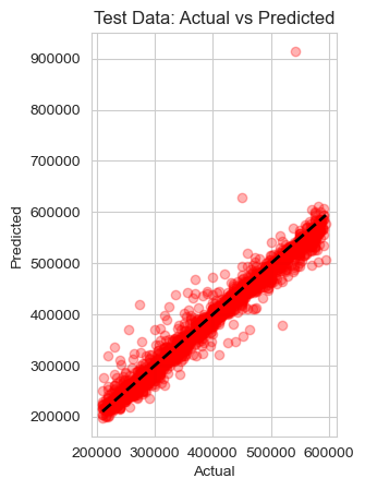
Figure 3. Prediction accuracy of Fcnn+cnn.

Based on the estimation results of the experiments, Figure 3 shows the scatter diagram of the property prices and the predicted values. It indicates that FCNN+CNN fits the data well in most cases. For extreme values, the model exhibits significant bias and performs poorly. Figure 4 illustrates the correlation between actual prices and predicted values. The majority of predicted values align closely with the red line, suggesting that the model fits the experimental data accurately.

Then comes the Generative Adversarial Fully Connected Networks (FCNN+GANs). Its chimerism R² score for the dataset is 0. 5223, and then MAE, and RMSE are 49783, and 61295 respectively under the same evaluation criteria. This shows that the performance of FCNN+GANs on this data is also a rather average situation, even inferior to the FCNN model alone.

The next one is Generative Adversarial Fully Connected Convolutional Networks (FCNN+GANs+CNN). In the base model, this model offers an R² of 0. 97 for the test dataset, while the MAE, and RMSE are 17235, and 27289 respectively. It is clear that this model is also well suited for the experimental data.

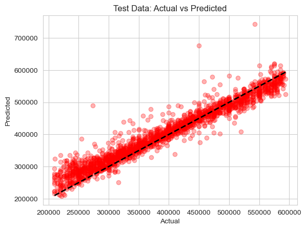
Figure 4. Model accuracy of Fcnn+cnn+Gans

In most cases, FCNN+GANs+CNN also fit the data accurately (see Figure 4). However, the model performs poorly with high bias on some extremums in the middle and posterior part, where several points (room values > 65k) are far from the actual values. For the rest of the hairline, the model achieves a very ideal model fit, as most of the predicted results are very close to the actual values, but its performance is slightly inferior to FCNN+CNN with respect to the MSE and RMSE criteria.

Figure 5. Stability of Fcnn+cnn

Figure 6. Stability of Fcnn+cnn+Gans

According to Figure 5, and Figure 6, in order to verify the stability of the neural network model, this study used the method of setting the random number seed and repeating the experiments for five independent experiments on FCNN+CNN and FCNN+GANs+CNN models, respectively. This approach allows for consistent initial conditions for each experiment, which allows for a more reliable assessment of the model's performance across runs. The results show that the FCNN+CNN and FCNN+GANs+CNN models exhibit better stability across multiple experiments, which indicates that these models possess relatively good consistency and reliability under different data samples. Therefore, it is difficult for us to judge which specific model is the best, because the output of the model is related to the data set. To provide fast and accurate predictions and assistance to real estate price estimators, there are many factors to consider, including but not limited to the complexity and size of the data set, the complexity of the model and the running time. Therefore, if there are high requirements for accuracy, FCNN+GANs+CNN is a better choice, and this model has a stronger generalization ability and can provide more accurate predictions when the data set is small or the data features are very limited. If the data set is large or even increasing, and the accuracy requirements are not particularly stringent, FCNN+CNN is a better choice because it also has a very good accuracy rate, and is more lightweight and concise and can complete the task faster.

5. Conclusion

In this study, experiments were conducted to explore the enhancement effect of CNN feature extraction on neural network models based on Pytorch implementation. Through a series of experiments, this study finds that the introduction of CNN for feature extraction significantly enhances the performance of the FCNN model and its variant models. Specifically, the FCNN+CNN model was formed by combining CNN with FCNN and further combined with GANs to form the FCNN+GANs+CNN model. The experimental results show that these models exhibit excellent performance and stability in several evaluation metrics. In particular, the FCNN model based on CNN feature extraction shows significant improvement in metrics such as chimerism, MAE, and RMSE. The average results of several experiments show that the accuracy of the FCNN+CNN model and FCNN+GANs+CNN model reaches 97. 00% and 96. 56%, respectively, which is significantly better than the traditional FCNN model. Through this series of studies, the effectiveness of CNN in feature extraction is successfully verified and its great potential in enhancing the performance of neural network models is demonstrated. In summary, the CNN feature extraction method implemented based on Pytorch significantly enhances the performance of neural network models and provides strong support for subsequent research and applications.

However, there are still some shortcomings in this experiment: The dataset of this experiment has a total of about 15k samples and more outliers with larger fluctuations, and a small number of high-priced outliers are deleted because of the larger impact on model prediction, which reacts to the lack of maturity of this study's model in the handling of outliers. The number of cycles of the stability assessment is less, and the model stability is not sufficiently demonstrated. The data variety is not enough, and we can consider adding the Icon image data to further utilize the CNN feature extraction capability. In addition, the real house price data has been more volatile in recent years, with more outliers and noise, so the next step can be to work on better analysis and prediction of the noise outliers.

References

[1]. Kaur H, Kushwanth A, Akshay Y and Kiran Y 2023 Real Estate Forecasting System Using Machine Learning Algorithms Proc. 2023 6th Int. Conf. on Contemporary Computing and Informatics (IC3I) vol 6 (New York: IEEE) pp 25–29
[2]. Ho W K, Tang B S and Wong S W 2021 Predicting property prices with machine learning algorithms J. Property Res. 38(1) 48–70
[3]. Hinton G E, Deng L, Yu D and others 2021 A comprehensive review on deep learning architectures and their applications IEEE Trans. Neural Netw. Learn. Syst. 32(4) 1130–46 https://doi.org/10.1109/TNNLS.2021.3051345
[4]. Taye M M 2023 Theoretical understanding of convolutional neural network: Concepts, architectures, applications, future directions Computation 11(3) 52 https://doi.org/10.3390/computation11030052
[5]. Nirthika R, Manivannan S, Ramanan A and others 2022 Pooling in convolutional neural networks for medical image analysis: a survey and an empirical study Neural Comput. Applic. 34 5321–47 https://doi.org/10.1007/s00521-022-06953-8
[6]. Waldmann P 2019 On the Use of the Pearson Correlation Coefficient for Model Evaluation in Genome-Wide Prediction Front. Genet. 10 Article 499 https://doi.org/10.3389/fgene.2019.00899
[7]. Waoo A A and Soni B K 2021 Performance Analysis of Sigmoid and Relu Activation Functions in Deep Neural Network (Singapore: Springer) pp 39–52 https://doi.org/10.1007/978-981-16-2248-9_5
[8]. Nirthika R, Manivannan S, Ramanan A and Wang R 2022 Pooling in convolutional neural networks for medical image analysis: a survey and an empirical study Neural Comput. Applic. 34(7) 5321–47
[9]. Dundar A and Culurciello E 2014 Flattened convolutional neural networks for feedforward acceleration arXiv:1412.5474
[10]. Zhang W, Liu H, Li B, **e J, Huang Y, Li Y and others 2024 Dynamically masked discriminator for GANs Adv. Neural Inf. Process. Syst. 36
[11]. Karras T, Laine S and Aila T 2019 A style-based generator architecture for generative adversarial networks Proc. IEEE/CVF Conf. on Computer Vision and Pattern Recognition (CVPR) pp 4401–10
Cite this article
Zhang,J. (2024). Application and Performance Comparison of Compound Neural Network Model based on CNN Feature Extraction in House Price Forecast. Applied and Computational Engineering,96,210-217.
Data availability
The datasets used and/or analyzed during the current study will be available from the authors upon reasonable request.
Disclaimer/Publisher's Note
The statements, opinions and data contained in all publications are solely those of the individual author(s) and contributor(s) and not of EWA Publishing and/or the editor(s). EWA Publishing and/or the editor(s) disclaim responsibility for any injury to people or property resulting from any ideas, methods, instructions or products referred to in the content.
About volume
Volume title: Proceedings of the 2nd International Conference on Machine Learning and Automation
© 2024 by the author(s). Licensee EWA Publishing, Oxford, UK. This article is an open access article distributed under the terms and
conditions of the Creative Commons Attribution (CC BY) license. Authors who
publish this series agree to the following terms:
1. Authors retain copyright and grant the series right of first publication with the work simultaneously licensed under a Creative Commons
Attribution License that allows others to share the work with an acknowledgment of the work's authorship and initial publication in this
series.
2. Authors are able to enter into separate, additional contractual arrangements for the non-exclusive distribution of the series's published
version of the work (e.g., post it to an institutional repository or publish it in a book), with an acknowledgment of its initial
publication in this series.
3. Authors are permitted and encouraged to post their work online (e.g., in institutional repositories or on their website) prior to and
during the submission process, as it can lead to productive exchanges, as well as earlier and greater citation of published work (See
Open access policy for details).