1. Introduction

Artificial intelligence (AI) is an increasingly developing field, which is applied to simulate human behaviors, analyze data, make judgments, and enhance from experience automatically [1]. Machine learning (ML) has emerged as an attractive solution to large-scale problems, such as Image recognition and classification [2], natural language processing, medical diagnosis [3]. ML algorithms, including classification, clustering, regression, association rule mining, and reinforcement learning, have been widely used in many application domains [1]. The basic rules on ML are shown as follow. To sum up, the problem of machine learning can be separated into the training and the prediction phase (seen from Fig. 1) [4]. Due to the need for processing large-scale data and complex models that exceed the computational capacity of a single machine, leveraging multiple computing resources to accelerate training and enhance scalability, distributed machine learning emerged. Advances in network communication, distributed storage systems, and the rise of edge computing further enabled its development. There are two essentially distinct approaches to dividing the problem among all processors when it comes to distribution: parallelizing the data or the model as depicted in Fig. 2 [4, 5].

As previously indicated, distributed learning can handle vast data sets that cannot be stored and processed on a single system by utilizing parallel processing resources to solve large-scale issues in a reasonable amount of time. First, one looks at algorithms designed to be run on a single computer. Distributed machine learning (DML) has seen significant advancements driven by the increasing need to process vast datasets and complex models that exceed the capabilities of single machines. Early research focused on the scalability challenges, leading to the development of frameworks such as Google’s TensorFlow and Apache Spark that allow distributed computing across clusters of machines. These frameworks enable parallelization of both data and model computation, thus accelerating training times [6].

Key progress has been made in optimization techniques specific to distributed environments. Algorithms like Distributed Stochastic Gradient Descent (DSGD) have been enhanced to reduce communication overhead, a major bottleneck in distributed learning. Techniques such as model averaging, local updates, and asynchronous updates have been widely studied to improve convergence rates without overwhelming network bandwidth [7]. The rise of edge computing and federated learning has introduced new dimensions to distributed learning. Federated learning, in particular, allows training on decentralized data sources, such as mobile devices, while preserving privacy. Research in this area has focused on challenges like communication efficiency, security, and heterogeneity in data distribution [8]. Moreover, distributed learning's application in large-scale deep learning models, such as GPT-3 and BERT, highlights the importance of balancing computation and communication. Recent work has explored how distributed architectures can support models with billions of parameters, pushing the boundaries of what is computationally feasible.

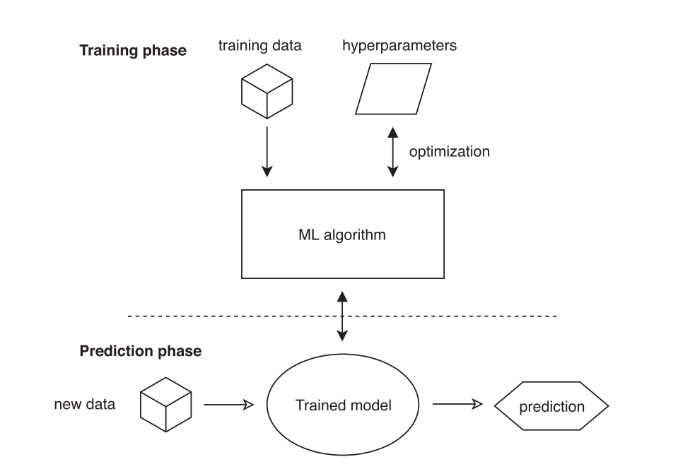
Figure 1. Training and prediction phase [4].

Recently, both business and academics have shown a great deal of interest in distributed machine learning schemes like federated learning (FL) because of the growing concerns about privacy and communication limitations. Training a global model with weights x is the aim of FL. To do this, it must solve the following optimization problem.[8]

\( min_{x}F(x)=\frac{1}{m}Σ_{i=1}^{m}f_{i}(x)\ \ \ (1) \)

When training an optimization process, a loss function measures the difference between the goal value and the anticipated output of the model. The kind of work at hand and the characteristics of the data being used will determine which loss function is best. Several popular loss functions that are appropriate for various machine learning applications and goals are mean squared error (MSE), mean absolute error (MAE), hinge loss, and cross-entropy loss. For Lipschitz smooth definition, f is L-smooth if ||∇f(x)−∇f(y)||2≤L||x−y||2||∇f(x)−∇f(y)||2​≤L||x−y||2​ for all x, y. L-smooth indicates that the gradient of a function does not change too abruptly, or that the function is smooth. During the research, this study has carried out the models. Theoretically, more local update leads to lower accuracy, and strong heterogeneity leads to lower accuracy and poor error convergence (high error floor), However, in the situation, larger τ instead have lower error floor across the board. Probable cause is that the dataset does not meet the requirements for Lipschitz smooth, so the conclusion Larger τ gives worse error convergence” may not hold in this particular case. Next, this study will try some more datasets to find a Non-Lipschitz smooth function, analyze how the number of iteration τ changes affects the accuracy of the training.

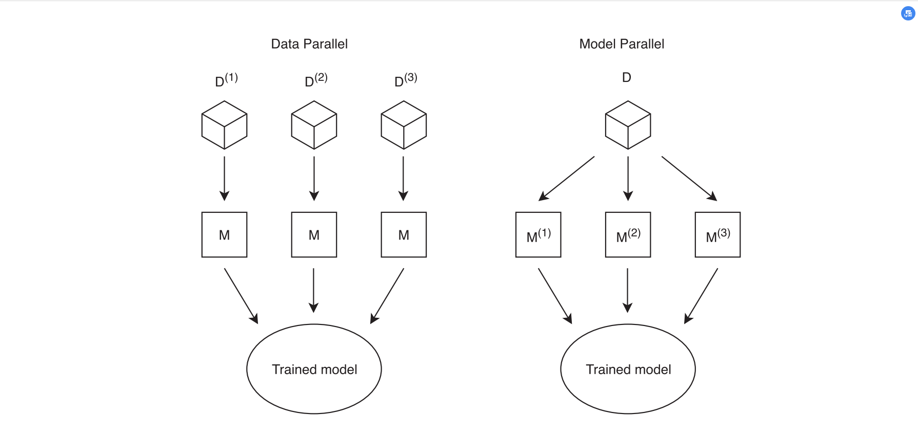
Figure 2. Data and model parallel [4].

2. Data and method

Three datasets will used. The first is phone user’s information with data volume of 320k, feature dimension of 25 dimensions; predicted label category of 9 categories. The goal is to predict the mobile phone usage habits of different users based on their behaviors, thus recommending different types of cellular plan for them. Datasets 2 is the CSGO Pro Players Datasets with feature dimension of 20 dimensions. One acquired the demofiles from the popular CSGO fan site, HLTV.org. As a personal fan of CSGO's competitive circuit, this study decided to extract out data of 803 pro players from HLTV for model training. This study used csgo demofiles from matches until 2nd May, 2022. This research thrilled to introduce the Ultimate Music Analysis Dataset, a comprehensive collection of 2,000 songs, providing a rich resource for music enthusiasts, data analysts, and researchers delving into the intricacies of musical composition and trends. This dataset is an invaluable resource for anyone looking to explore the diverse and fascinating world of music, offering a detailed look at the elements that contribute to the art and science of song creation and popularity [9, 10].

Eminem is one of the most influential hip-hop artists of all time, and the Rap God. This study acquired this data using Spotify APs and supplemented it with other research to add to my own analysis. This study has primarily used data from Spotify’s API using multiple endpoints for albums and tracks. This research supplemented the data with stats from Billboard and calculations from this post. One will see new visualizations using this data or using the sales, swear, or duration for an analysis.

An artificial neural network (ANN) is a computational model designed to simulate the human brain. Similar to biological neurons in the brain, ANNs consist of artificial neurons, which serve as processing units, and they are extensively interconnected. One of the key capabilities of an ANN is its ability to generalize, meaning it can produce accurate outputs for unseen inputs by learning from examples. The main features of ANNs include learning from data, the non-linearity of processing elements, adaptability, parallelism in processing, and fault tolerance. In multidimensional space, neural networks are viewed as universal approximators of data, capable of achieving both local and global approximations. The multilayer perceptron (MLP) is the most prominent example of a global network within ANNs, utilizing a sigmoidal activation function for its neurons. The MLP structure consists of layers of neurons arranged in a hierarchy, starting from the input layer, moving through one or more hidden layers, and ending at the output layer. Connections are only allowed between neurons in adjacent layers. The structure of an MLP is characterized by:

• Input layer: Receives the input data.

• Hidden layers: Perform computations and iterative optimizations.

• Output layer: Provides the final predicted outcome.

This architecture allows MLPs to solve complex nonlinear problems and exhibit strong learning and adaptation capabilities, making them highly effective in various predictive and classification tasks [11].

The initial goal of the gradient boosting approach was very high prediction accuracy. Nevertheless, the algorithm's capacity to generate decision trees in a sequential manner posed challenges to its extensive implementation. Because every tree is built to fix every mistake committed by its predecessors, even simple models take a long time to train. As a result, the training time was ineffective. The procedure was expedited using the potent algorithm eXtreme Gradient Boosting (XGBoost), allaying these worries. To parallelize data organization and build trees separately, XGBoost makes advantage of several cores. Consequently, this leads to much shorter search times and faster model training, which ultimately improves performance [12]. This particular strategy was selected because of several advantages (a) addressing missing values; (b) necessitating data scaling; (c) suggesting a computationally effective variation of the gradient boosting approach; (d) yielding good results in machine learning contests and being effectively used in other research and fields [13, 14]. For every dataset, this study will use one algorithm to train, change the iteration time, and try to find out the result whether the differences between loss function type (L-smooth or Non-L-smooth) do impact error convergence.

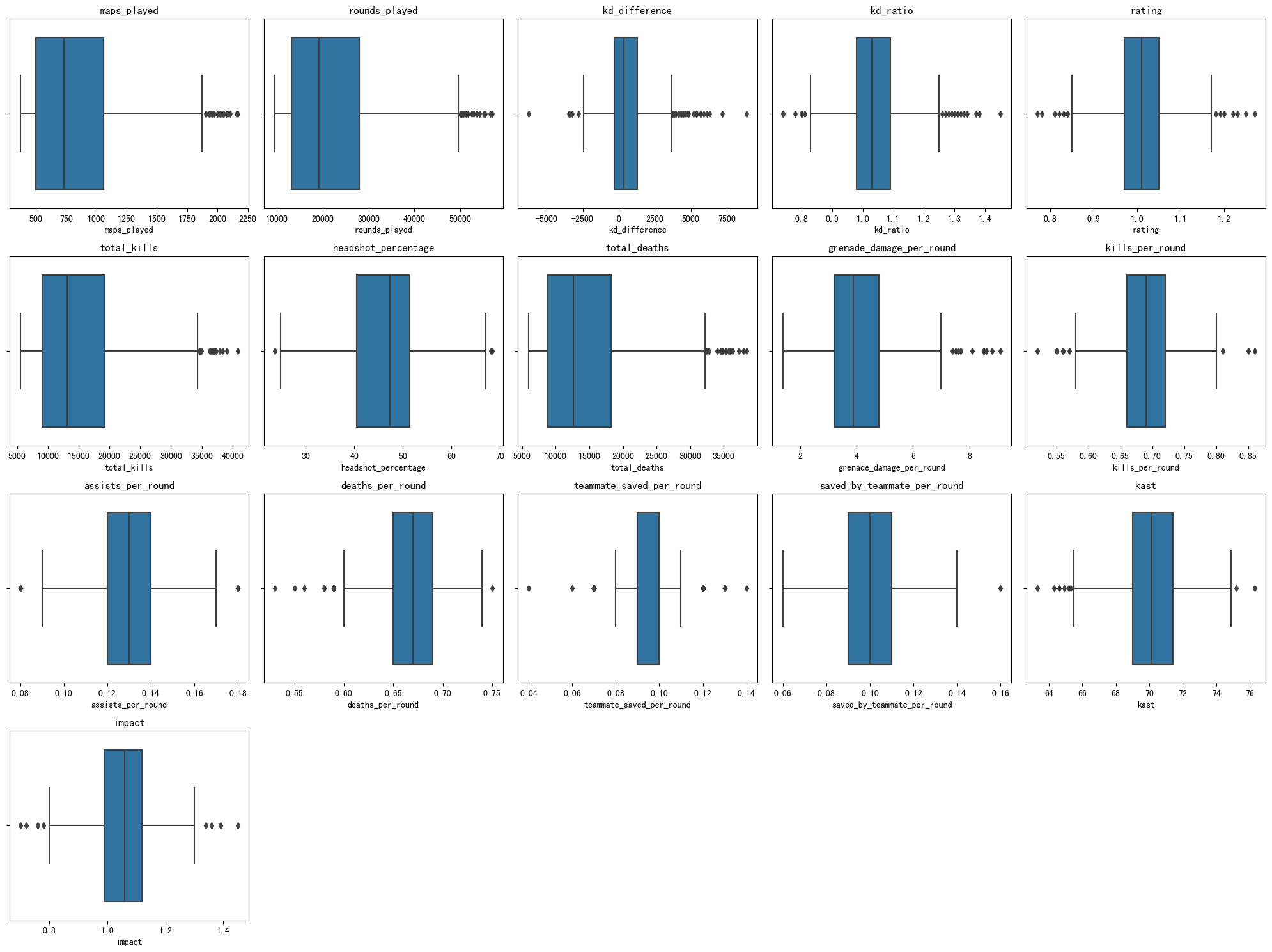
Figure 3. Boxplot for datasets 2 (Photo/Picture credit: Original).

3. Results and discussions

3.1. Data cleaning

For Dataset1, to initialize the data heterogeneity, one has two experimental methods. First method used is that Each data set still includes the original 9 categories, but the proportion of each category are different. The second method is non-overlapping splitting that a dataset only includes a few categories. For example, this research will totally have 9 categories overall, the first data set include the first four categories while the second data set includes the other five categories. These two data sets don’t meet each other to initialize the data heterogeneity. This structure is actually in line with the actual production background, such as two companies, their data are private and do not share with each other. Dataset 2 contains 803 records and 20 fields. None of the fields have missing values. The data type also appears to be appropriate, but some fields, such as Teams, may require further processing to accommodate the machine learning model. Next, the following steps are carried out, i.e., check the basic statistics of the numeric field to identify any possible outliers and check the unique values of categorical fields, such as country and teams, to ensure that they are suitable for model training. This study uses a boxplot to identify possible outliers. One can then decide what to do with these values as shown in Fig. 3. The Datasets contains 2000 records and 18 fields. None of the fields have missing values. The data type also looks appropriate. One can observe outliers in some features, especially in features such as loudness and popularity. Outliers can be handled in a variety of ways, including deleting, replacing, or retaining. Here, given the size of the dataset and the needs of the machine learning model, this study will replace the outliers with the median of each feature. Outliers are generally defined as values less than the first quartile minus a 1.5-fold interquartile range (IQR) or greater than the third quartile minus a 1.5-fold IQR. This research will follow this definition to identify and handle outliers shown in Fig. 4.

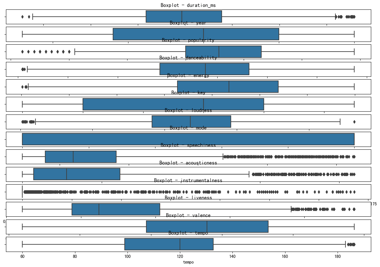
Figure 4. Boxplot for datasets 3 (Photo/Picture credit: Original).

There are 20 missing values in the swear_words_album column in the data (seen from Fig. 5). This study is going to use the median of the swear_words_album column to fill in the missing values. Next, this study will make sure that all the data is numeric for easy processing of MLP and XGBoost models. This study is going to work with non-numeric data by following these steps:

• Convert the "explicit" column to a numeric (0 or 1).

• Remove the "id" column because it's an identifier and generally doesn't help the model make predictions.

• Convert the album_released and album_peaked_on columns to timestamps.

• Remove the available_markets, name, and album_name columns, as they are text data and are not suitable for direct use in model training.

• The comma in "total_sales_US" is stripped and converted to a numeric type.

The final split ratio is Training Set: Validation Set: Test Set = 70%:15%:15%.

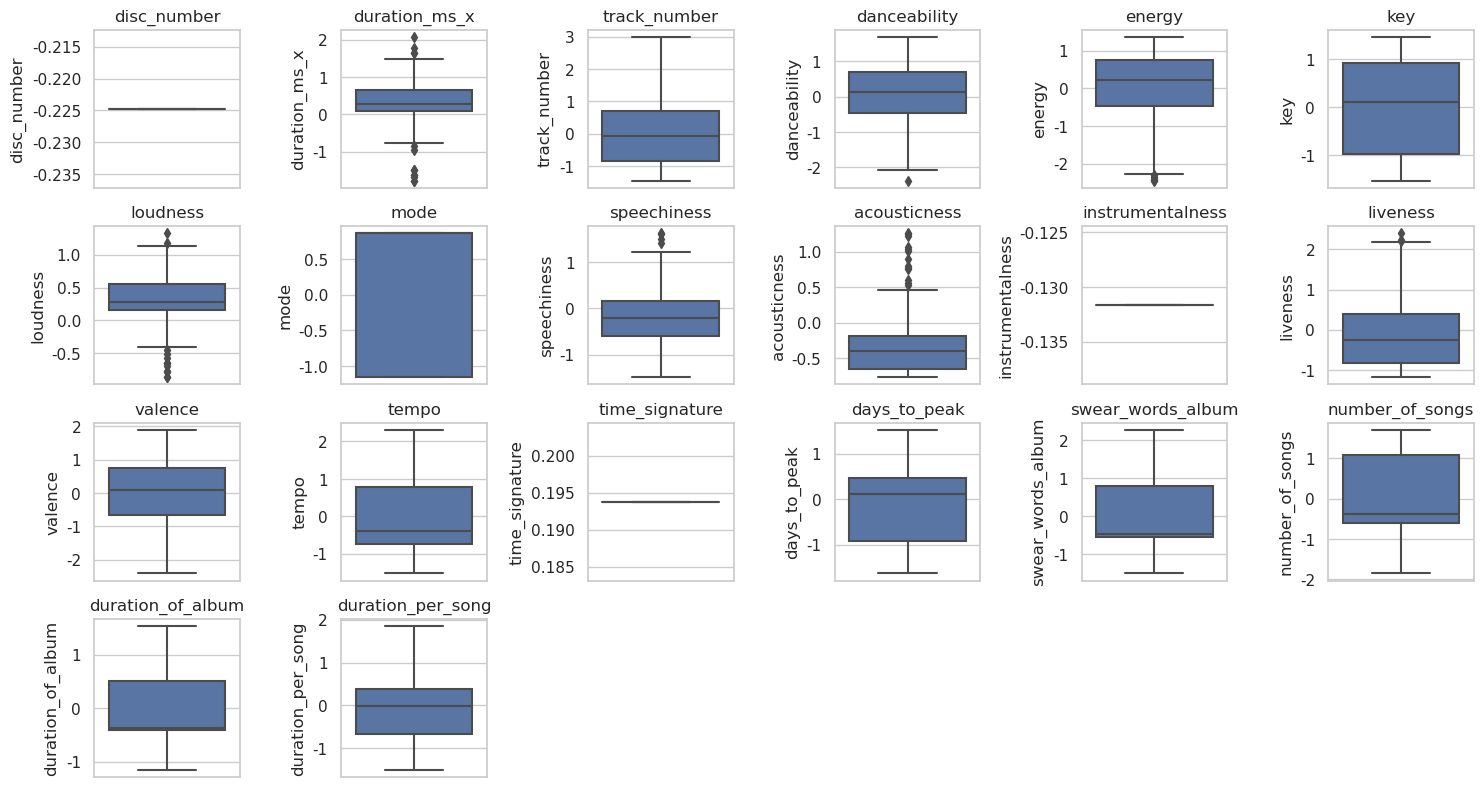
Figure 5. Boxplot for variables in datasets 3 (Photo/Picture credit: Original).

3.2. Model performances

Using a three-layer neural network structure, the number of nodes in the input layer is determined according to the number of data features, which is the number of other columns excluding the Teams column after the one-hot encoding. If model complexity is complex, the hidden layer is set up to three layers, the first hidden layer is set up with 256 neurons, the second hidden layer is set up with 128 neurons, and the last layer is set up with 64 neurons. Otherwise, the hidden layer is set up to two layers, the first hidden layer is set up with 128 neurons, and the second hidden layer is set up with 64 neurons. The number of nodes in the output layer depends on the specific task, for example, if it is a classification task, the number of nodes in the output layer can be set to the number of categories.

During training, the back propagation algorithm is used to calculate the gradient of the loss function to the model parameters. Model parameters are updated with SGD, adjusting them based on the direction and size of the gradient to gradually reduce the loss function. To observe the effect of the number of iterations on the error convergence, one can choose different loss functions, such as mean square error (L-smooth) or cross-entropy (Non-L-smooth). Gradually, this study will increase the number of iterations and observe the changes in the loss function to determine the convergence speed and stability of the model. For dataset2, first this study used TensorFlow's Sequential model to build a three-layer MLP model consisting of two hidden layers and an output layer. Compile using the SGD optimizer and binary_crossentropy loss function. Then, the training set is used for training, and changes in loss and accuracy are recorded during training. Finally, the loss and accuracy curves are plotted to observe the training effect of the model. The parameters are as follows: Epochs=200,batch size=16,optimizer='SGD', loss='binary_crossentropy'. As one can see, Train Accuracy, loss functions type (use mean squared error (L-smooth) and cross-entropy (Non-L-smooth) and Validation Accuracy remain the same from the beginning. Afterward, one will change the Epochs and batch size, it also didn’t change at all as depicted in Fig. 6.

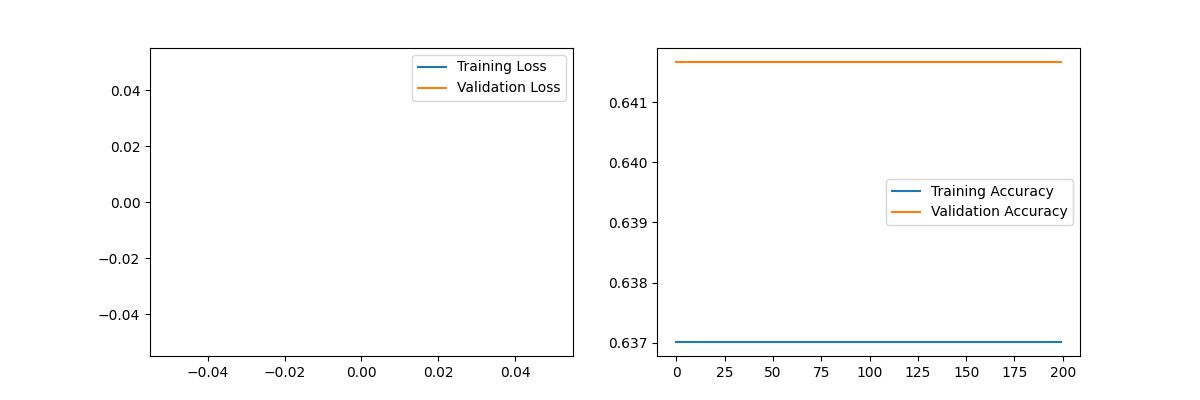
Figure 6. Loss and accuracy for dataset2 (Photo/Picture credit: Original).

For dataset3, this study began by cleaning the raw data and also added new features for text length, such as the number of characters in the artist and song names. After cleaning, the dataset was split into features (X) and target (y), with a 20% test split. This research then standardized the feature values using StandardScaler to ensure proper scaling. For the model, this study implemented a Multi-Layer Perceptron (MLP) using the MLPRegressor from Scikit-learn with parameters such as hidden layers of sizes (64, 32), ReLU activation, SGD optimizer, and an adaptive learning rate. The model was trained with varying iteration counts (100, 500, and 1000) to analyze how error convergence changes. Eventually, one visualized the mean squared errors for both the training and testing sets across different iteration counts to study the impact on model performance. As one can see from Fig. 7, larger iteration leads to lower error convergence (for L-smooth: MSE), which is expected. Next, one will change the loss function type (Non-L-smooth: Huber Loss).

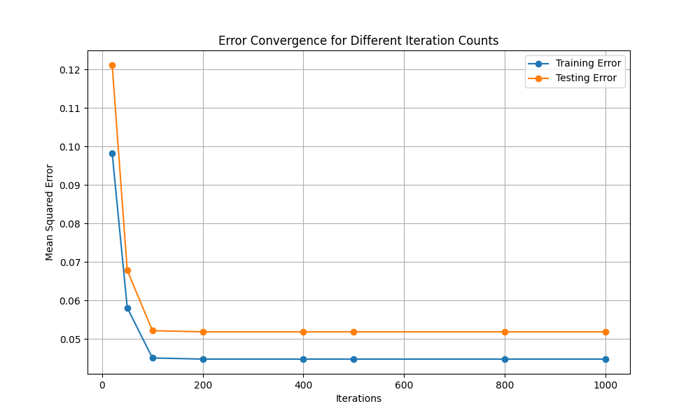
Figure 7. Error convergency for dataset3 (Photo/Picture credit: Original).

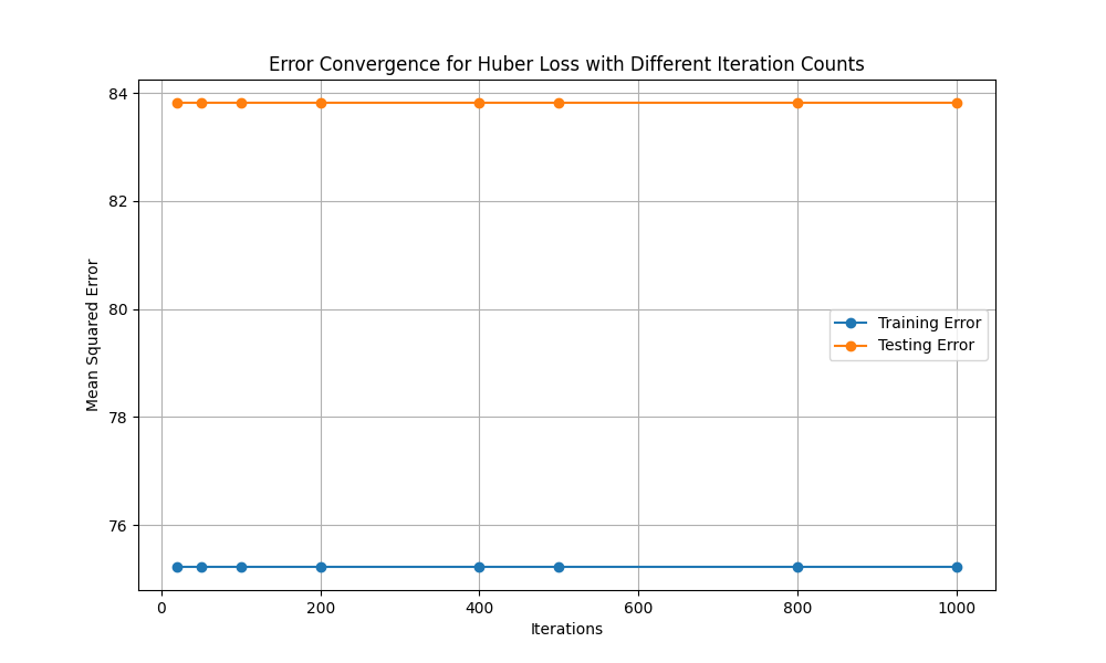
Figure 8. Error convergency of Huber Loss for dataset3 (Photo/Picture credit: Original).

As presented in Fig. 8, error convergence for Huber Loss doesn’t change almost with larger iteration. The possible reason may be the data is relatively clean, less noisy, and has a more uniform distribution of errors, and the MSE may be good enough to handle errors. In this case, changing the loss function will not have much of an impact on the error convergence. The main purpose of Huber Loss is to smooth out large points of error, and if there are not many outliers in the data, the effect of Huber Loss may not be obvious. To deal with that issue, this study will adjust the epsilon parameter: lower the epsilon value so that Huber Loss switches to the MAE section earlier, and see if it has a more obvious effect on large error points. The epsilon parameter adjustment is from 1.35 to 1.00. The impact is getting more obvious as given in Fig. 9. Because the data is too clean after cleaning, the difference is not very noticeable. Heever, one can see that with larger iteration, the error convergence is getting larger. Hence, one can draw the conclusion. For Non-L-smooth loss function, with larger iterations, the error convergence will be larger relatively.

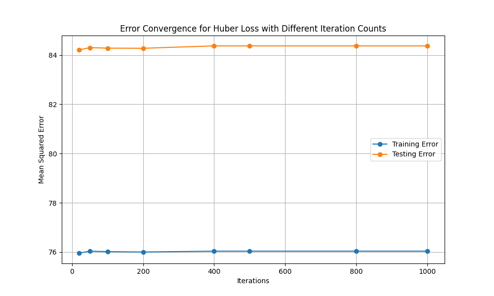
Figure 9. Error convergency of Huber Loss for dataset3 with epsilon parameter (Photo/Picture credit: Original).

For XGBoost setup, the learning rate is 0.1, the max depth is 3, the number of estimators is 100. One needs to create an XGBoost classifier using the configured hyperparameters. One can use gradient boosting to optimize performance, train the model on the training set, and evaluate it on the validation set. This research needs to observe the influence of different loss functions (error and log loss) on error convergence by plotting the evaluation metric curves during training. Then, this study will vary the iteration count for XGBoost training (5,10,20,50,100,200) and observe the changes in model performance by also plotting the corresponding curves in Fig. 10.

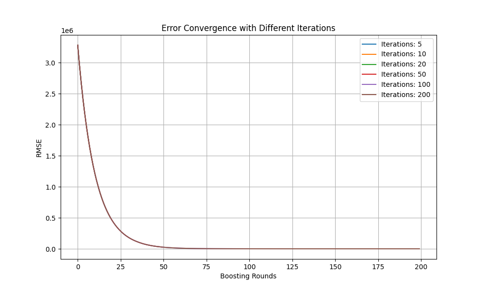
Figure 10. Error convergency for XGBoost (Photo/Picture credit: Original).

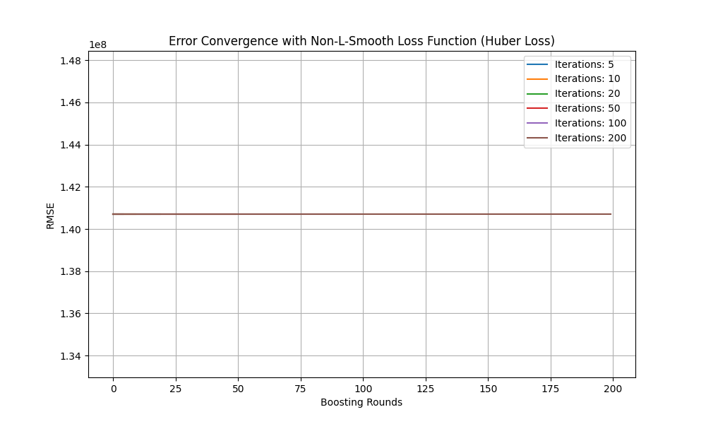
Figure 11. Error convergency for XGBoost of Huber Loss (Photo/Picture credit: Original).

As one can see, larger iteration leads to lower error convergence (for L-smooth: MSE), which is expected. Next, one changes the loss function type (Non-L-smooth: reg: pseudo Huber error). The parameters are iteration_counts = [5,10,20,50,100,200], learning_rate=0.1, and max_depth=3. Seen from Fig. 11, it remains the same. Similar results (illustrated in Fig. 12) are obtained with parameters iteration_counts = [5,10,20,50,100,200]; learning_rate=0.05; max_depth=5,; objective='reg:pseudohubererror' (Non-L-smooth Loss Function) and MAE was used as metric.

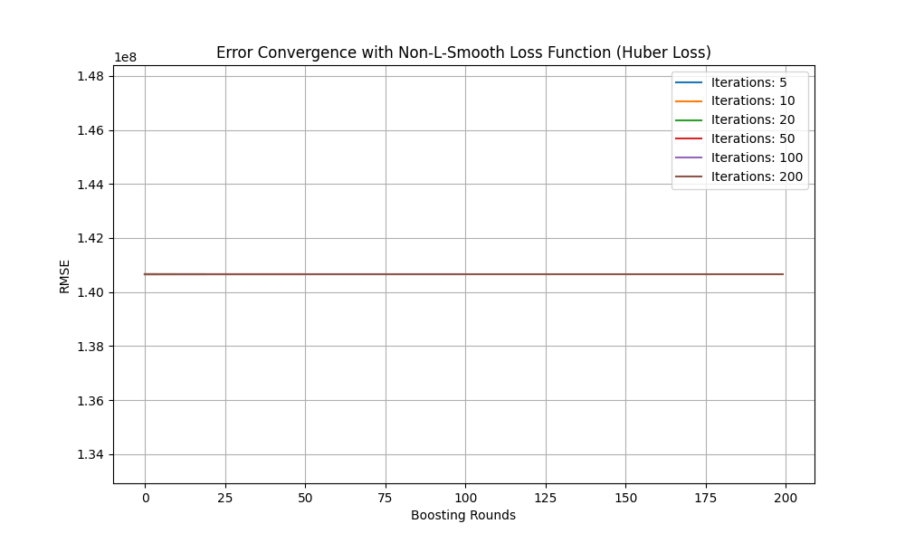
Figure 12. Error convergency for XGBoost of Huber Loss with different parameters (Photo/Picture credit: Original).

3.3. Limitation and prospects

Through the previous research, one has indeed explored the change of error convergence in deep learning for the choice of different loss functions (L-Smooth or Non-L-Smooth) with the increase of the number of iterations. But there are several possible reasons why the experimental results are not so obvious. The dataset may be very small or there isn't enough complexity and variability in the data, and through data cleaning efforts, the data is too clean and inherently unsuitable for training and testing. If the model has already overfitted the training data, further iterations will not improve the error on the validation set, but may instead increase. If the model is not complex enough (for example, too shallow in depth or too low in learning rate), the model will not be able to capture patterns in the data, even if the number of iterations is increased. Maybe the model has already achieved optimal error convergence at an earlier stage, the increased number of iterations or the adjustment of the loss function will not have much effect. The model may have converged to the local optimal solution.

For future prospects one can increase model complexity, i.e., increase hidden layers or adjust the number of neurons to see if one can speed up convergence or help better handle complex data. It is necessary to check the dataset in order to confirm that the dataset is complex enough, large enough, and has some non-trivial patterns and variations. One can check the number of outliers and large error data points in the data. If there are fewer outliers, Huber Loss does not significantly alter convergence. Meanwhile, it is necessary to adjust the complexity of the model with cross-validation to avoid overfitting or underfitting.

4. Conclusion

To sum up, the pursuit of error convergence is significant for machine learning. In addition, the number of iterations will directly affect it. In this paper, by selecting different datasets and using two different algorithms, MLP and XGBoost, the influence of different loss function types on the error convergence under the condition of increasing iterations is discussed. Experiments show that the error convergence of the L-smooth loss function is smaller with the increase of the number of iterations, while the Non-L-smooth loss function is the opposite: with the increase of the number of iterations, the error convergence is greater. In the future, larger datasets will be selected, and more complex models will be used for training after more accurate cleaning, so as to improve the accuracy of the research.

References

[1]. Dehghani M and Yazdanparast Z 2023 From distributed machine to distributed deep learning: a comprehensive survey Journal of Big Data vol 10(1) p 158
[2]. Bojarski M 2016 End to end learning for self-driving cars arXiv preprint arXiv:160407316
[3]. Khandani A E, Kim A J and Lo A W 2010 Consumer credit-risk models via machine-learning algorithms Journal of Banking & Finance vol 34(11) pp 2767-2787
[4]. Verbraeken J, Wolting M, Katzy J, Kloppenburg J, Verbelen T and Rellermeyer J S 2020 A survey on distributed machine learning Acm computing surveys (csur) vol 53(2) pp 1-33
[5]. Peteiro-Barral D and Guijarro-Berdiñas B 2013 A survey of methods for distributed machine learning Progress in Artificial Intelligence vol 2 pp 1-11
[6]. Xing E P, Ho Q, Xie P and Wei D 2016 Strategies and principles of distributed machine learning on big data Engineering vol 2(2) pp 179-195
[7]. Khromov G and Singh S P 2023 Some intriguing aspects about lipschitz continuity of neural networks arXiv preprint arXiv:230210886
[8]. Pan L and Song S 2023 Local SGD accelerates convergence by exploiting second order information of the loss function arXiv preprint arXiv:230515013
[9]. Bian W and Chen X 2012 Smoothing neural network for constrained non-Lipschitz optimization with applications IEEE transactions on neural networks and learning systems vol 23(3) pp 399-411
[10]. Osowski S, Siwek K and Markiewicz T 2004 June MLP and SVM networks-a comparative study Proceedings of the 6th Nordic Signal Processing Symposium 2004 NORSIG 2004 pp 37-40
[11]. Desai M and Shah M 2021 An anatomization on breast cancer detection and diagnosis employing multi-layer perceptron neural network (MLP) and Convolutional neural network (CNN Clinical eHealth vol 4 pp 1-11
[12]. Ramraj S and Uzir N Sunil R Banerjee S 2016 Experimenting XGBoost algorithm for prediction and classification of different datasets International Journal of Control Theory and Applications vol 9(40) pp 651-662
[13]. Torlay L, Perrone-Bertolotti M, Thomas E and Baciu M 2017 Machine learning–XGBoost analysis of language networks to classify patients with epilepsy Brain informatics vol 4 pp 159-169
[14]. Dhaliwal S S, Nahid A A and Abbas R 2018 Effective intrusion detection system using XGBoost Information vol 9(7) p 149
Cite this article
Wu,D. (2024). Comparison Impacts of Iteration Quantities on Loss Function for Different Data Sets. Applied and Computational Engineering,96,68-78.
Data availability
The datasets used and/or analyzed during the current study will be available from the authors upon reasonable request.
Disclaimer/Publisher's Note
The statements, opinions and data contained in all publications are solely those of the individual author(s) and contributor(s) and not of EWA Publishing and/or the editor(s). EWA Publishing and/or the editor(s) disclaim responsibility for any injury to people or property resulting from any ideas, methods, instructions or products referred to in the content.
About volume
Volume title: Proceedings of the 2nd International Conference on Machine Learning and Automation
© 2024 by the author(s). Licensee EWA Publishing, Oxford, UK. This article is an open access article distributed under the terms and
conditions of the Creative Commons Attribution (CC BY) license. Authors who
publish this series agree to the following terms:
1. Authors retain copyright and grant the series right of first publication with the work simultaneously licensed under a Creative Commons
Attribution License that allows others to share the work with an acknowledgment of the work's authorship and initial publication in this
series.
2. Authors are able to enter into separate, additional contractual arrangements for the non-exclusive distribution of the series's published
version of the work (e.g., post it to an institutional repository or publish it in a book), with an acknowledgment of its initial
publication in this series.
3. Authors are permitted and encouraged to post their work online (e.g., in institutional repositories or on their website) prior to and
during the submission process, as it can lead to productive exchanges, as well as earlier and greater citation of published work (See
Open access policy for details).