1. Introduction

With the acceleration of urbanization and population growth, traffic congestion has become increasingly severe. Intelligent Transportation System is an indispensable part of smart city, and traffic flow prediction is an essential component of Intelligent Transportation System. Accurate traffic flow prediction is crucial for alleviating congestion, optimizing route planning, and guiding vehicle dispatch [1]. Traditional statistical methods and machine learning techniques, such as linear regression, decision trees, and support vector machines, often require extensive feature engineering and parameter tuning, making it difficult to effectively handle the complex spatio-temporal dependencies and external factors affecting traffic data [2]. In recent years, deep learning technology has made significant progress in the field of traffic flow prediction due to its powerful feature extraction and pattern recognition capabilities. By learning the features and complex patterns in the data, deep learning models can capture non-linear relationships and dynamic changes in time series, achieving more accurate predictions. However, existing deep learning models also have certain limitations. Most models require a large amount of data to achieve good performance, and the computational complexity of these models is relatively high.

Despite the extensive research on the application tasks of traffic flow prediction in existing literature, there is a notable absence of in-depth analysis in the summarization and categorization of related content. Furthermore, the analysis of the advantages and disadvantages of these models is insufficient. This deficiency hinders a comprehensive understanding of the real-world performance and limitations of different models.

This paper provides an overview of deep learning models for traffic flow prediction. It begins by classifying the tasks and common data representations. We then introduce and compare various models, including CNNs, GCNs, RNNs, attention mechanisms, and hybrid models, highlighting their advantages and disadvantages. Suggestions for improvement and optimization are provided for each model's limitations. The paper concludes by discussing the challenges and future research directions in the field.

2. Traffic flow prediction preparation

2.1. Task

In traffic flow prediction, there are many aspects involved in application tasks [3], which are as follows:

Firstly, predict the number of vehicles passing through a specific road segment within a unit of time based on historical traffic flow data. Secondly, pay attention to the real-time speed of vehicles, which is usually derived from vehicle sensor data or camera data. Then, forecast the travel demand volume in a certain area at a future time step based on historical travel data. It is also necessary to predict potential traffic incidents, such as traffic congestion and accidents. There are various external information factors that interfere with the prediction of actual traffic data, such as weather changes, points of interest, holidays, etc., so considering the impact of external information is crucial. Finally, based on the above predictive analysis, optimize route selection to provide the best solution for travelers (Figure 1).

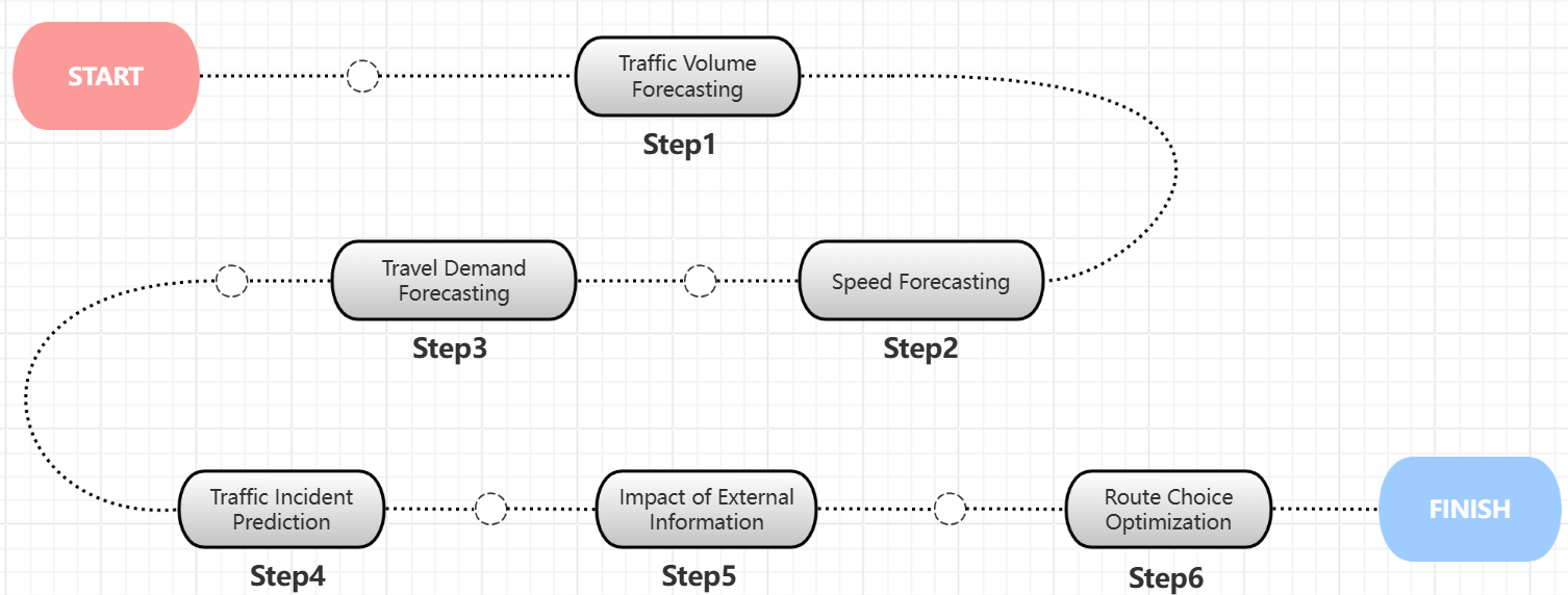
Figure 1. Flow chart of the application task of traffic prediction [3]

2.2. Data

Table1 shows the common data representation forms.

Table 1. Common data representation forms

Paper [4] provided sources of traffic data acquisition, and mainly focused on traditional machine learning methods (Figure 2).

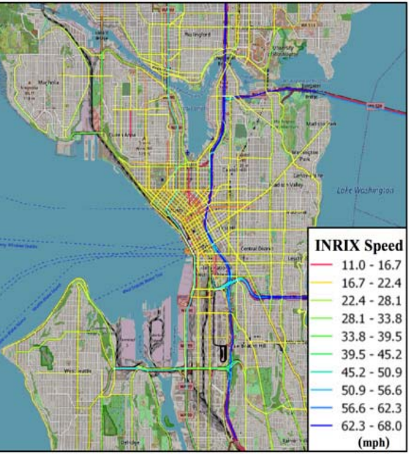
Figure 2. An example of a Traffic Network Graph [4]

In response to a series of application tasks and data processing in traffic flow prediction, deep learning methods can better meet the requirements. Therefore, through continuous exploration and improvement, a multitude of models based on deep learning have been developed. The following diagram is a general classification framework (Figure 3).

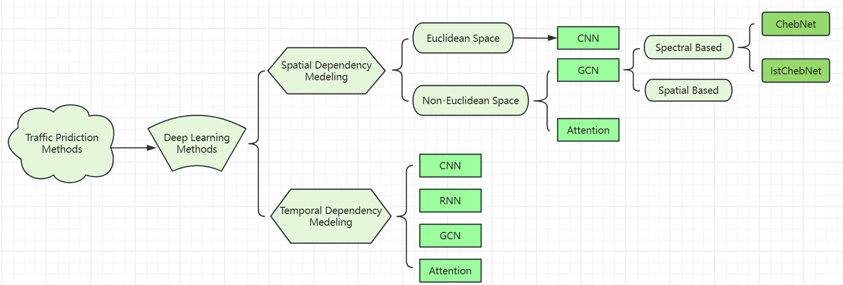
Figure 3. Mind map for classification of deep learning models in traffic flow prediction [3]

Next, we will provide a detailed explanation of each fundamental deep learning method, introduce their basic principles, analyze their respective advantages and limitations, propose some related optimization strategies, and offer prospects for the future.

3. Model analysis and evaluation

3.1. Spatial dependency model

3.1.1. Euclidean space Based on Euclidean space, a spatial-dependent CNN [5] model is commonly used. The core idea is to convert traffic flow data into a two-dimensional matrix and utilize the convolutional and pooling layers of CNN to extract spatial features from the traffic flow data, such as the correlation of flow between adjacent observation points. Subsequently, the fully connected layers integrate the extracted features and output the final prediction results. This model is capable of effectively capturing the spatial variation patterns in traffic flow data, thereby enhancing the accuracy of traffic flow predictions.

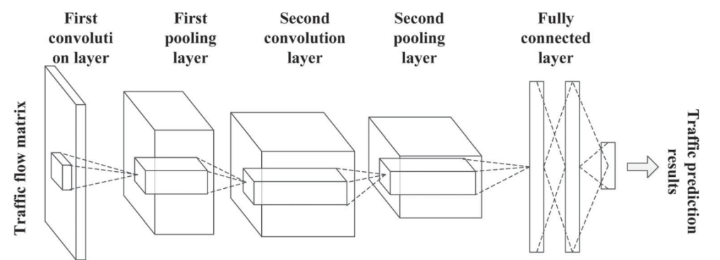
Figure 4. Schematic structure of the CNN [6]

In paper [6], a short-term traffic flow prediction model based on a CNN deep learning framework for spatial analysis is described. Figure 4 shows a simplified framework of CNN. It demonstrates the complete process from traffic flow matrix to predicted results. First, the data enters the first convolution layer, followed by the pooling layer, then the second convolution layer and another pooling layer. Finally, this information goes through the fully connected layer to produce the predicted results. The article employs a model that combines CNN with STFSA (Spatial-Temporal Feature Selection Algorithm), and the results indicate that this model achieved the highest prediction accuracy in both single-step and multi-step prediction tasks. Firstly, CNN effectively extracts spatiotemporal features from traffic data, learning nonlinear patterns for precise predictions. Moreover, the paper employs methods such as L2 regularization and batch processing to prevent model overfitting and to enhance the model's generalization capabilities.

Certainly, the spatial-dependent CNN model has its limitations. The model primarily focuses on the spatial features of traffic flow data, neglecting temporal correlations. For instance, it may fail to capture the flow variations during peak and off-peak periods. The model assumes that the traffic network is a Euclidean space. However, in real-world traffic networks, the distance between traffic observation points may be influenced by factors such as terrain, road network structure, and cannot be simply measured by Euclidean distance. The model is also sensitive to outliers. Sudden events like traffic congestion, accidents, or other emergencies can lead to abnormal fluctuations in traffic flow data.

Paper [7] proposes a multi-feature prediction model based on CNN, named MF-CNN. It combines multiple spatiotemporal features and external factors, making the analysis more comprehensive and the prediction more accurate. In the paper, traffic flow data from 8 adjacent time intervals are used as the input for short-term features, and traffic flow data from 7 consecutive days and 2 consecutive weeks are used as the input for long-term features, considering various spatiotemporal features. The JPEA dataset is used to demonstrate the impact of weather and holidays as external factors on traffic flow. The MF-CNN model adopts an end-to-end learning structure, integrating feature extraction, feature fusion, and prediction output into a single model, simplifying the training and prediction process.

3.1.2. Non-euclidean space Based on non-Euclidean space, a method that typically combines spatial dependency GCN [8] with attention mechanisms is adopted. The principle lies in simulating the spatial dependency relationships in traffic networks through a graph structure, where GCN propagates information between nodes on the graph, using an adjacency matrix to weight and aggregate node features, thereby capturing the interactions between nodes in irregular traffic networks. The Attention mechanism [9], on the other hand, calculates the correlation weights between nodes, dynamically emphasizing the spatial relationships that are more critical to the prediction results, allowing the model to focus on the more important connection paths in the traffic network. These two methods collectively demonstrate the capability of handling complex spatial dependencies in non-Euclidean spaces, free from the limitations of traditional Euclidean distances, and can better adapt to the diversity and irregularity of actual traffic networks.

In paper [10], a deep learning model called ASTGCN is proposed, which integrates GCN and attention mechanisms for traffic flow prediction (Figure 5). ASTGCN combines multi-source data to capture spatio-temporal patterns using graph convolution and attention, followed by a fully connected layer for refinement. Experiments on two real-world highway datasets show that ASTGCN outperforms existing benchmark models in prediction accuracy. GCN captures spatial relationships, while the attention mechanism dynamically adjusts node weights, effectively capturing dynamic spatio-temporal correlations. Additionally, ASTGCN extracts features directly from raw data, simplifying the training process and reducing human-induced errors. The attention matrix provides an intuitive understanding of each sensor's influence on the prediction results.

Certainly, the ASTGCN model has its shortcomings. The model includes multiple hyperparameters such as the order of Chebyshev polynomials and the size of convolutional kernels. The selection of these hyperparameters can make the model overly sensitive to their values. The computational complexity of GCN and the attention mechanism is high, leading to longer training and prediction times, especially in large-scale traffic networks. Lastly, when the connections between nodes in the traffic network are sparse, the information that GCN can obtain from each node is limited, which affects performance. Therefore, this model is not suitable for handling sparse data.

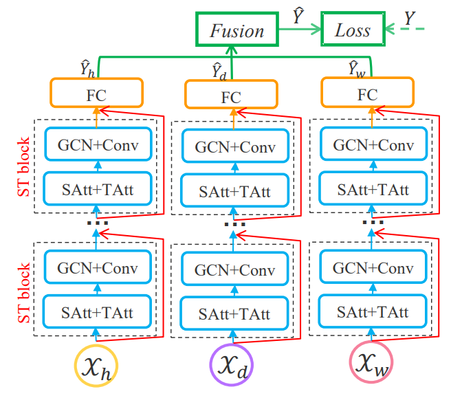
Figure 5. The framework of ASTGCN. SAtt: Spatial Attention; TAtt: Temporal Attention GCN: Graph Convolution; Conv: Convolution; FC: Fully-connected; ST block: SpatialTemporal block [10].

To address the sparsity of spatial dependencies, we can adopt the STGNN (Spatial Temporal Graph Neural Network) model introduced in paper [11] for processing. The positional attention mechanism in STGNN can dynamically adjust the importance of neighboring nodes based on node features, effectively capturing complex relationships between nodes even in sparse data. Furthermore, STGNN can automatically adapt to the structural features of sparse data through the learning process, enabling better learning of the intrinsic features of the data and thus avoiding overfitting.

3.2. Temporal dependency model

Deep learning methods based on temporal dependency primarily focus on the dynamic relationships between different time points in time series data, thereby capturing the patterns of traffic flow variation over time. These methods mainly include CNN, RNN, GCN, and Attention mechanisms.

CNN extracts local features from time series data, such as periodicity and trends, through convolutional layers and pooling layers. Convolutional layers use learnable convolutional kernels to slide over the time dimension, performing a weighted sum of data from adjacent time points to extract local features. Pooling layers then reduce the dimensionality of the features extracted by the convolutional layers while retaining the most important information.

RNN [12] captures the long-term dependencies in time series data by taking the output from the previous time point as input to the current time point through recurrent units. These units typically contain a hidden state that stores information from past time points. The principle of GCN is to capture the spatial dependencies between nodes through a graph structure, but it can also be extended to temporal dependencies. T-GCN introduces the time dimension into the graph convolution process, using time convolutional layers or time encoders to capture the trend of node features changing over time. Attention mechanism can dynamically adjust the weights of relevance between different elements in a sequence, focusing on elements that have a greater impact on the prediction results. It helps the model capture key information in time series data and improves prediction accuracy.

In addition, these methods can also be used in combination, and their selection should be based on their respective characteristics and advantages, as well as the specific application scenarios and task requirements.

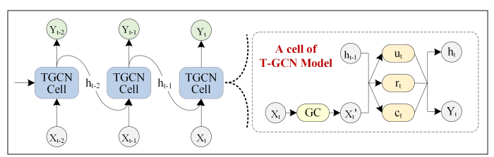
Figure 6. The overall process of spatio-temporal prediction. The right part represents the specific architecture of a T-GCN unit, and GC represents graph convolution [13].

In paper [13], the application of the T-GCN model in traffic prediction is specifically described. By combining GCN and GRU(a variant of RNN), the model is designed to capture spatial and temporal dependencies, respectively. Figure 6 shows the overall process of the T-GCN model described in a previous paper you sent me. The model processes input data \( {X_{t}} \) , \( {X_{t-1}} \) , and \( {X_{t-2}} \) through a series of T-GCN Cells, each containing a graph convolution layer and a gated recurrent unit. These cells sequentially receive hidden states \( {h_{t-2}} \) , \( {h_{t-1}} \) from the previous time step and the current input data, and after processing, output new hidden states \( {h_{t}} \) as well as prediction values \( {Y_{t}} \) , \( {Y_{t+1}} \) , and \( {Y_{t+2}} \) . In addition, the bottom right corner of the picture enlarges the specific structure of a TGCN cell, including steps such as input merging, graph convolution operations, and state updates.Experiments conducted on two real-world traffic datasets (SZ-taxi and Los-loop) show that the T-GCN model outperforms other baseline methods in terms of prediction accuracy.

The T-GCN model achieved a reduction in RMSE of 30.62% and 30.32% for 15-minute and 30-minute traffic prediction tasks, respectively, compared to the GCN model that only considers spatial features. It also reduced RMSE by 1.82% and 3.12% compared to the GRU model that only considers temporal features. This demonstrates the significant advantage of the T-GCN model in capturing both temporal and spatial dependencies simultaneously. The paper presents the trends of RMSE and Accuracy for the T-GCN model across different prediction time horizons, showing that its prediction results are relatively stable, indicating its suitability for long-term traffic prediction.Furthermore, a perturbation analysis experiment was conducted by adding Gaussian noise and Poisson noise to the dataset. The results show that the T-GCN model's prediction accuracy changes little, indicating strong robustness to noise interference.

However, the T-GCN model performs poorly in predicting local extreme, such as peak traffic during rush hours. This may be due to the smoothing filter of the GCN model, which can smooth out the peaks. The paper also mentions that the "zero taxi value" phenomenon may lead to the misjudgment of non-zero road segments as zero in the traffic feature matrix, thus affecting the prediction accuracy of the T-GCN model. Moreover, the paper does not provide detailed information on the training and prediction time of the T-GCN model. Nevertheless, based on its model structure and complexity, it can be inferred that the computational cost is likely to be high, which may make it less suitable for scenarios with limited resources.

Paper [14] presents the Long Short-Term Memory (LSTM) [15], a model based on RNN. Its characteristic is the ability to capture long-term dependencies in time series and effectively learn nonlinear features in traffic flow. This enables LSTM to have a certain capability to predict local extrema, compensating to some extent for the shortcomings of T-GCN. Moreover, compared to T-GCN, the model structure of LSTM is simpler, the training process is relatively easy, and the computational efficiency is relatively higher.

4. Experimental comparative analysis

Based on the experimental data of each model on different datasets in the table 2, the following comparative analysis is conducted:

Among the models based on Euclidean space, the MAPE of CNN+STFSA is relatively small. This is because the CNN part can effectively extract spatial features from traffic flow data, while STFSA can help the model capture the dynamic changes of time series, which contributes to maintaining a lower relative error overall. However, its MAE is relatively large, which may be due to the model's sensitivity to outliers and its suboptimal performance in handling extreme values or noise in the data. On the other hand, MF-CNN significantly outperforms CNN+STFSA in terms of both MAE and RMSE. It considers both short-term and long-term features of the data, and this multi-scale feature fusion can more comprehensively capture the changing patterns of traffic flow. More importantly, it takes into account the interference of various external factors such as weather, holidays, and points of interest, which can all affect the prediction results.

Table 2. Comparison of prediction results among different deep learning models

In the models based on non-Euclidean space, it can be observed that the indicators of STGNN are significantly lower than those of ASTGCN. This is likely because GCN is not suitable for processing sparse data. When the connectivity between nodes in the traffic network is sparse, the performance of GCN is affected. However, in STGNN, the importance of neighboring nodes can be dynamically adjusted based on their features, allowing it to effectively capture complex relationships between nodes even in sparse data.

In terms of temporal dependency models, T-GCN shows significantly better prediction performance than LSTM. T-GCN combines GCN and GRU, enabling it to capture both spatial and temporal dependencies, making it suitable for long-term traffic prediction and providing a more comprehensive overall performance. LSTM can capture long-term dependencies in time series, making it suitable for predicting local extrema and complementing the shortcomings of T-GCN. However, it is not as comprehensive as T-GCN.

5. Conclusion

This study reviews the application of deep learning models in traffic flow prediction, categorizing them into spatial dependence models and temporal dependence models based on their dependencies. Spatial dependence models are further divided into Euclidean and non-Euclidean types, with representative models from each category introduced along with their advantages and disadvantages.The analysis indicates that CNNs are suitable for handling data based on Euclidean space, significantly improving prediction accuracy by integrating multiple spatiotemporal features. The combination of GCNs and attention mechanisms effectively addresses data in non-Euclidean spaces by capturing spatial relationships between nodes in the traffic network and dynamically adjusting the weights between nodes. In cases of sparse connectivity, STGNNs can be employed, utilizing a positional attention mechanism to dynamically adjust the importance of neighboring nodes. For temporally dependent data, T-GCNs can simultaneously capture both spatial and temporal dependencies, while LSTMs can be employed to predict peak traffic flows, compensating for the limitations of T-GCNs.

Despite the significant progress made by deep learning models in traffic flow prediction, several challenges and future research directions remain. Firstly, there is a need to improve data quality and quantity, as well as to develop more effective methods for handling missing values, outliers, and noise. Secondly, the computational cost of some deep learning models, such as T-GCN, can be high, making them unsuitable for resource-constrained scenarios; hence, there is a demand for the development of lighter models that are more efficient. Thirdly, integrating multiple data sources, including traffic flow, weather, and road information, can greatly benefit traffic flow predictions, and thus, there is an urgent need to explore more effective multi-source data fusion techniques to enhance prediction accuracy. Lastly, the black-box nature of deep learning models makes it difficult to understand the prediction results, calling for the creation of more transparent models that allow for better insight into the prediction process and the influencing factors.

References

[1]. Nguyen, H., Kieu, L. M., Wen, T., et al. (2018). Deep learning methods in transportation domain: A review. IET Intelligent Transport Systems, 12(9), 998-1004. https://doi.org/10.1049/iet-its.2017.0536
[2]. Lv, Y., Duan, Y., Kang, W., et al. (2014). Traffic flow prediction with big data: A deep learning approach. IEEE Transactions on Intelligent Transportation Systems, 16(2), 865-873. https://doi.org/10.1109/TITS.2014.2306224
[3]. Yin, X., Wu, G., Wei, J., et al. (2021). Deep learning on traffic prediction: Methods, analysis, and future directions. IEEE Transactions on Intelligent Transportation Systems, 23(6), 4927-4943. https://doi.org/10.1109/TITS.2020.3014229
[4]. Nagy, A. M., & Simon, V. (2018). Survey on traffic prediction in smart cities. Pervasive and Mobile Computing, 50, 148-163. https://doi.org/10.1016/j.pmcj.2018.06.003
[5]. Alzubaidi, L., Zhang, J., Humaidi, A. J., et al. (2021). Review of deep learning: Concepts, CNN architectures, challenges, applications, future directions. Journal of Big Data, 8, 1-74. https://doi.org/10.1186/s40537-021-00449-7
[6]. Zhang, W., Yu, Y., Qi, Y., Shu, F., & Wang, Y. (2019). Short-term traffic flow prediction based on spatio-temporal analysis and CNN deep learning. Transportmetrica A: Transport Science, 15(2), 1688–1711. https://doi.org/10.1080/23249935.2018.1547045
[7]. Yang, D., Li, S., Peng, Z., et al. (2019). MF-CNN: Traffic flow prediction using convolutional neural network and multi-features fusion. IEICE TRANSACTIONS on Information and Systems, 102(8), 1526-1536. https://doi.org/10.1587/transinf.2019EDL8003
[8]. Danel, T., Spurek, P., Tabor, J., et al. (2020). Spatial graph convolutional networks. In International Conference on Neural Information Processing (pp. 668-675). Cham: Springer International Publishing. https://doi.org/10.1007/978-3-030-59923-9_61
[9]. Niu, Z., Zhong, G., & Yu, H. (2021). A review on the attention mechanism of deep learning. Neurocomputing, 452, 48-62. https://doi.org/10.1016/j.neucom.2021.02.078
[10]. Guo, S., Lin, Y., Feng, N., et al. (2019). Attention based spatial-temporal graph convolutional networks for traffic flow forecasting. In Proceedings of the AAAI Conference on Artificial Intelligence (Vol. 33, pp. 922-929). https://doi.org/10.1609/aaai.v33i01.3301922
[11]. Wang, X., Ma, Y., Wang, Y., et al. (2020). Traffic flow prediction via spatial temporal graph neural network. In Proceedings of the Web Conference 2020 (pp. 1082-1092). https://doi.org/10.1145/3366423.3380379
[12]. Sherstinsky, A. (2020). Fundamentals of recurrent neural network (RNN) and long short-term memory (LSTM) network. Physica D: Nonlinear Phenomena, 404, 132306. https://doi.org/10.1016/j.physd.2020.132306
[13]. Zhao, L., Song, Y., Zhang, C., et al. (2019). T-GCN: A temporal graph convolutional network for traffic prediction. IEEE Transactions on Intelligent Transportation Systems, 21(9), 3848-3858. https://doi.org/10.1109/TITS.2019.2923473
[14]. Fu, R., Zhang, Z., & Li, L. (2016). Using LSTM and GRU neural network methods for traffic flow prediction. In 2016 31st Youth Academic Annual Conference of Chinese Association of Automation (YAC) (pp. 324-328). IEEE. https://doi.org/10.1109/YAC.2016.7475848
[15]. Hochreiter, S., & Schmidhuber, J. (1997). Long short-term memory. Neural Computation, 9(8), 1735-1780. https://doi.org/10.1162/neco.1997.9.8.1735
Cite this article
Guo,X. (2024). Research on Deep Learning Models for Traffic Flow Prediction. Applied and Computational Engineering,111,87-96.
Data availability
The datasets used and/or analyzed during the current study will be available from the authors upon reasonable request.
Disclaimer/Publisher's Note
The statements, opinions and data contained in all publications are solely those of the individual author(s) and contributor(s) and not of EWA Publishing and/or the editor(s). EWA Publishing and/or the editor(s) disclaim responsibility for any injury to people or property resulting from any ideas, methods, instructions or products referred to in the content.
About volume
Volume title: Proceedings of CONF-MLA 2024 Workshop: Mastering the Art of GANs: Unleashing Creativity with Generative Adversarial Networks
© 2024 by the author(s). Licensee EWA Publishing, Oxford, UK. This article is an open access article distributed under the terms and
conditions of the Creative Commons Attribution (CC BY) license. Authors who
publish this series agree to the following terms:
1. Authors retain copyright and grant the series right of first publication with the work simultaneously licensed under a Creative Commons
Attribution License that allows others to share the work with an acknowledgment of the work's authorship and initial publication in this
series.
2. Authors are able to enter into separate, additional contractual arrangements for the non-exclusive distribution of the series's published
version of the work (e.g., post it to an institutional repository or publish it in a book), with an acknowledgment of its initial
publication in this series.
3. Authors are permitted and encouraged to post their work online (e.g., in institutional repositories or on their website) prior to and
during the submission process, as it can lead to productive exchanges, as well as earlier and greater citation of published work (See
Open access policy for details).