1. Introduction

Maps are a necessary tool for the study of marine science. Usually, the accuracy of the generated map depends largely on the accuracy of the underwater vehicle positioning. Underwater scenes are full of restrictions, for example, GPS (Global Positioning System), which is commonly used by ground and air robots is less useful underwater as AUVs cannot obtain GPS information due to the strong attenuation of underwater electromagnetic waves, which brings great challenges to the navigation of autonomous underwater vehicles. In the absence of GPS, acoustic positioning systems or positioning systems based on inertial information are commonly used. However, for deep-sea areas, the operating distance of conventional underwater acoustic navigation is limited and the mother ship needs to follow or arrange acoustic beacons in advance, which is not suitable for use in unknown areas of the sea. The individual inertial navigation will produce cumulative errors over time and the accuracy of the estimation will gradually decrease. Although GPS correction algorithms at regular sea level can constrain cumulative errors, it is difficult to achieve accuracy in deep-sea measurement tasks.

Compared with acoustic and inertial positioning systems, Simultaneous Localisation and Mapping (SLAM), as an autonomous navigation technology, can fuse inertial navigation information and DVL and the Kalman filter to eliminate cumulative errors. This can provide reliable positioning for autonomous underwater vehicles (AUVs) in an unknown environment during movement and generate a model of their surrounding environment. Underwater SLAM provides a safe, efficient and economical method for exploring and investigating unknown underwater environments. With the development and utilisation of underwater resources such as oceans, underwater SLAM has become a research hotspot.

Underwater SLAM can be divided into three categories according to the type of sensor: visual SLAM, light detection and ranging (LiDAR) SLAM and sonar SLAM. Laser radar uses a laser to analyse the contour and structure of the target. However, electromagnetic waves cannot propagate long distances underwater, and the laser will be severely attenuated in the water, resulting in absorption and scattering. Although vision-based SLAM has the advantages of low cost and high portability, it has poor visibility in deep-sea environments and is affected by particle and light conditions in water. The lack of illumination will seriously affect the quality of the final image. Sonar can detect and locate objects in the absence of light by using the characteristics of the object’s reflected sound wave. The sound wave shows a smaller attenuation rate and longer propagation distance than light in the underwater environment. Although the refresh rate and resolution of the visual camera are lower, sonar is an ideal choice for underwater SLAM. The sonar sensors used for underwater SLAM mainly include mechanical scanning sonar, side scanning sonar, multi-beam sonar, etc.

Multi-beam sonar (MBS) is a kind of sonar used for underwater detection and it is one of the most important measuring instruments in ocean missions. Multi-beam sonar, which is widely used, can transmit hundreds of beams at the same time [1]. Cheng et al. proposed a filter-based multi-beam forward-looking sonar (MFLS) underwater SLAM algorithm [2]. In order to prevent excessive calculation, after extracting environmental features, threshold segmentation and distance constraint filtering are used and converted into sparse point cloud format. In addition, the method also combines multi-sensor data to estimate the position of the AUVs. The SLAM method based on Rao-Blackwellised particle filter (RBPF) can be used to generate a map [3].

When performing underwater SLAM, a single type of sensor has some disadvantages. Integrating multiple sensors can solve these disadvantages and improve the robustness and accuracy of underwater SLAM. Common multi-sensor fusion methods include visual-inertial SLAM, laser-visual SLAM and multi-sensor SLAM combining sonar, IMU, vision and other sensors.

In general, the computational complexity of the SLAM system is affected by the size of the exploration environment and is closely related to feature extraction, tracking, data association [6], filtering methods, etc. Due to the huge space of underwater environments, such as lakes and oceans, AUV activities are complex. Moreover, in the face of large-scale SLAM tasks, it is difficult to achieve a balance between accuracy and speed. Improving accuracy in large-scale environments is still an urgent problem to be solved in underwater SLAM applications.

Considering the principle of the SLAM system, the feature-matching and solution results of SLAM in dynamic environments will be affected. Therefore, for SLAM on land, its use in dynamic environments is a research hotspot [7, 8, 9]. Similarly, dynamic phenomena in underwater environments are very common, such as marine organisms, water flows caused by robot motions, bubbles, etc. Consequently, there are numerous defects and errors in the maps generated in dynamic environments.

Therefore, in response to the above challenges, this paper aims to develop a multi-AUV collaborative SLAM algorithm based on iUSBL. Our works aim to improve the reliability, continuity and robustness of AUV swarms in underwater pose estimation. Our research also seeks to improve the efficiency of underwater SLAM and generate more accurate and comprehensive map information for deep-sea navigation. Considering the dynamic underwater environment of the multi-AUV scene, the RANSAC algorithm is used to detect and eliminate dynamic points, which improves accuracy while ensuring efficiency and effectively suppresses the errors introduced by dynamic points.

2. Methodology

We proposed a multi-AUV collaborative SLAM algorithm based on iUSBL, which can effectively solve the problem of low efficiency of single AUV SLAM. The algorithm significantly improves the mapping efficiency and positioning accuracy through multi-AUV collaboration. Figure 1 is the overall framework of the collaborative SLAM algorithm proposed in this paper. The algorithm can be divided into three parts, the main AUV SLAM module, the slave AUV SLAM module and the map fusion module. The iUSBL is used for information exchange between the master and slave AUVs.

For a single AUV, the DVL data and IMU data are first fused to obtain the odometer data used for dead reckoning in the algorithm and the sonar data is processed. Firstly, threshold filtering is performed on the multi-beam sonar data and then it is converted into a point cloud form. Then, the RANSAC algorithm is used to eliminate the dynamic points. Finally, the distance constraint filtering is used to sparse the obtained point cloud data. The processed data is sent to the RBPF-SLAM algorithm for positioning and synthesis. The iUSBL is used for cooperative positioning between the master and slave AUVs and then the master and slave AUV maps are fused to generate the final map.

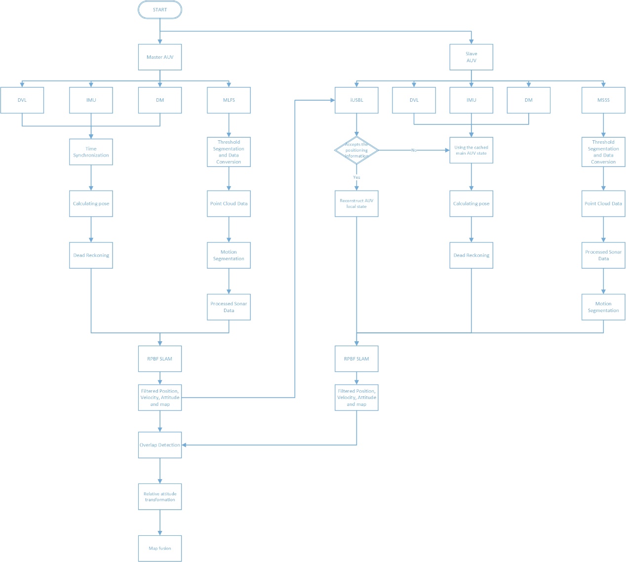
Figure 1: The overall framework of the collaborative SLAM algorithm.

2.1. iUSBL System

Compared with the traditional USBL system, the iUSBL system only needs to receive the signal from the AUV to the autonomous AUV, which avoids the multi-signal collision problem when multiple slave AUVs are located at the same time. Different from the traditional USBL, iUSBL is equipped with a beacon by the master AUV and a receiving array by the slave AUV to achieve one-way acoustic communication, which significantly reduces the communication energy consumption and time delay of the slave AUV. The iUSBL system is composed of a four-element transmitting array and a receiving hydrophone. The transmitting array is mounted on the master AUV, while the hydrophone is mounted on each slave AUV. The distance and azimuth between the master and slave AUVs can be calculated by receiving orthogonal coded signals from four arrays.

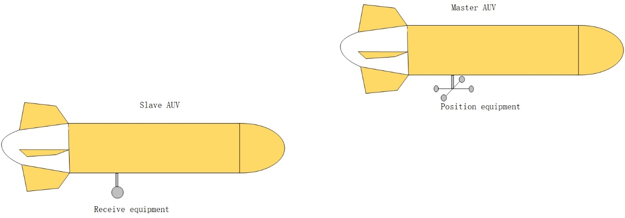
Figure 2: The iUSBL diagram between master and slave AUVs.

Due to the small size of the array, the distance between the receiving point and the transmitting end is far. It can be assumed that the sound lines are parallel. The relative azimuth angle between the master and slave AUVs is thus obtained:

\( cos{θ_{x}}=\frac{c∙{τ_{x}}}{L} \)

\( cos{θ_{y}}=\frac{c∙{τ_{y}}}{L} \)

L is the distance of the coaxial array, \( {θ_{x}} \) , \( {θ_{y}} \) are the target azimuth, \( {τ_{x}} \) , \( {τ_{y}} \) are the time delay difference.

The distance and relative position between the master and slave AUVs can be calculated based on the depth information of the depth sensor and the estimated azimuth information:

\( R=\frac{{z_{s}}-{z_{m}}}{\sqrt[]{1-{(cos{θ_{x}})^{2}}-{(cos{θ_{y}})^{2}}}} \)

\( x=R∙cos{θ_{x}} \)

\( y=R∙cos{θ_{y}} \)

In the formula, R is the target tilt distance, \( {z_{m}} \) , \( {z_{s}} \) are the depth information of the slave AUV, and x and y are the position of the slave AUV in the master AUV coordinate system. The master AUV broadcasts its coordinates regularly. According to the absolute position information of the main AUV and the relative position information between AUVs, each slave AUV is positioned by coordinate system transformation. The AUV position information is calculated from the measured values \( {z_{m}} \) , \( {z_{s}} \) , \( {τ_{x}} \) , \( {τ_{y}} \) . In these four measurements, the depth information \( {z_{m}} \) and \( {z_{s}} \) are obtained by the depth meter and the measurement accuracy is particularly high.

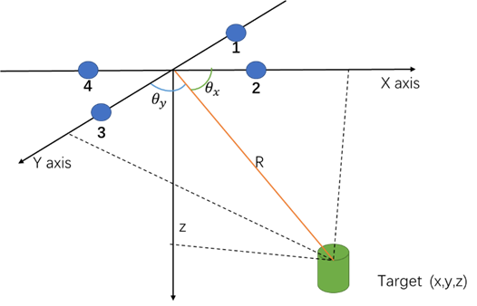
Figure 3: Geometric Graph of Theoretical Position.

2.2. Single AUV Dead Reckoning

The dead reckoning module uses IMU, DVL and DM to provide a rough estimation of AUV attitude. After sampling the data, the dead reckoning module uses the extended Kalman filter (EKF) to fuse the data of these sensors to estimate the attitude.

Because the depth measurement of DM is very accurate, the measured value of DM is regarded as the true value and only the two-dimensional plane needs to be considered when performing dead reckoning. The IMU includes an accelerometer and a gyroscope. The accelerometer detects the acceleration of the AUV along each axis, the gyroscope detects the angular velocity of the AUV relative to the navigation coordinate system and the DVL determines the speed of the AUV by measuring the Doppler effect of the underwater acoustic signal.

In this paper, the IMU / DVL tight coupling method is used to directly fuse the velocity information of DVL with the acceleration and angular velocity information of IMU. Compared with the loose coupling method, it can reduce the accumulation of navigation error more effectively, so as to improve the accuracy and stability of the whole system.

In order to achieve IMU / DVL tight coupling, we first need to convert the speed information of the DVL to the inertial coordinate system. This can be achieved by the following formula:

\( v_{DVL}^{n}=R({θ_{INS}})v_{DVL}^{b} \)

Thus, the calculation speed error:

\( {e_{v}}=v_{INS}^{n}-v_{DVL}^{n} \)

The position, velocity, attitude error and DVL drift are estimated and updated by Kalman filter. In the case of tight coupling, the velocity information of DVL is more effectively used to correct the error of INS..

2.3. Threshold Segmentation Algorithm

(1) The average pixel value of the sonar image is calculated as the threshold of filtering.

(2) The pixel value below the threshold is assigned to 0 and the pixel value above the threshold remains unchanged.

2.4. RANSAC Algorithm

(1) Select two adjacent frames of a sonar image and, according to the change of pixels in the sonar image in the sonar coordinate system, calculate the 3d flow across two frames.

(2) For a pair of matching feature points, the neighbours with similar 3D flow are selected as the cluster and the initial guesses of the rotation matrix R and the translation T are calculated. Based on the initial guess, the corresponding interior points are obtained. We will then iterate between the update R and T and the interior point until the interior point is no longer included. For a feature point, where we can’t find at least three similar neighbours, we will regard it as an outer point, skip and eliminate it.

(3) Select another pair of matching feature points from the remaining features and then proceed as described in step (4).

(4) After classifying all the features, the largest group is selected as the static group and the point cloud image after dynamic point elimination is generated.

2.5. RPBF-SLAM

Rao-Blackwellised PF-SLAM decomposes the SLAM problem into independent localisation and mapping. Its algorithm implementation is divided into four stages, the sampling stage, the weight calculation stage, the resampling stage and the map update stage:

(1) Sampling stage: for the particle set at time k, PF calculates the proposal distribution according to the motion model to obtain the particle set at time k + 1 and the pose of each particle represents a motion pose estimation of AUV.

(2) Weight calculation stage: the weight of each particle is \( \frac{1}{n} \) at the initial stage. After iterative updates, the weight is the ratio of the target distribution to the proposed distribution:

\( W_{k}^{i}=\frac{p(x_{1,k}^{i}|{z_{1:k}},{u_{1:k-1}})}{q(x_{1:k}^{i}|{u_{1:k-1}})} \)

(3) Resampling stage: resample the particle set according to the weight, discard the low weight and retain the high weight.

(4) Map update stage: particles update each feature in the map according to the sonar observation data and the current state trajectory.

3. Experimental Results

The simulation experiment was carried out using the ROS 2 platform. The Scott Reef 25 data set of the Australian Centre for Field Robotics’ marine robotics group was used. The effectiveness of the proposed SLAM algorithm was verified by simulation and practical experiments.

The experimental data was segmented to achieve the effect of multiple AUVs. The original trajectory was divided into five segments, assigned to five AUVs and then the data was grouped according to the trajectory, and the original data was divided into five parts. The trajectory of each AUV is shown below.

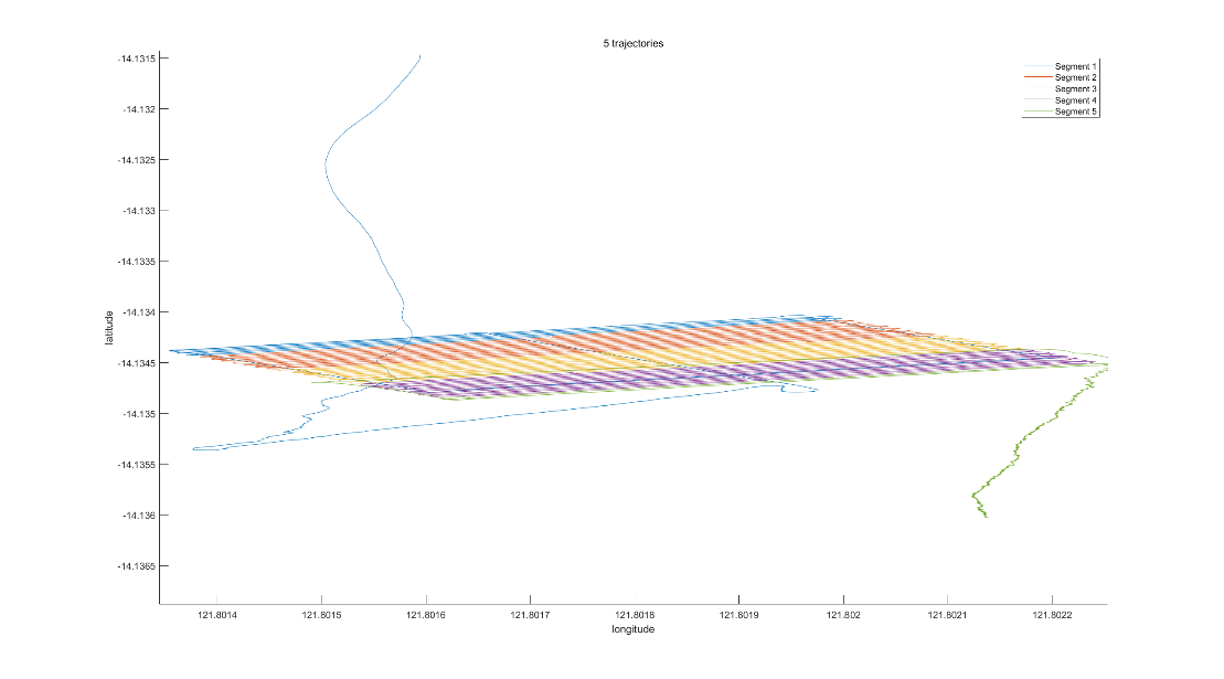
Figure 4: Trajectory segmentation results.

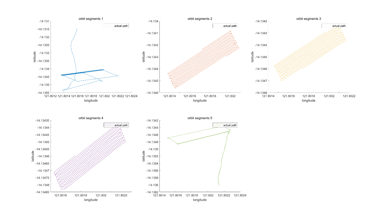
Figure 5: Trajectory corresponding to 5 AUVs.

3.1. Sonar Image Processing

The sonar image was processed by threshold filtering. Taking the previous two frames as an example, it can be seen that after threshold filtering, the noise of the sonar image was greatly reduced, which can better reflect the characteristics of the environment.

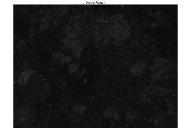
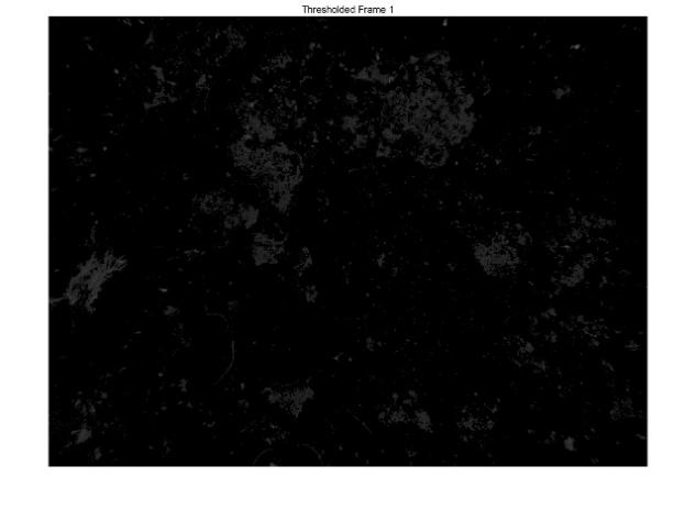
Figure 6: Comparison of the previous frame sonar image before and after threshold filtering.

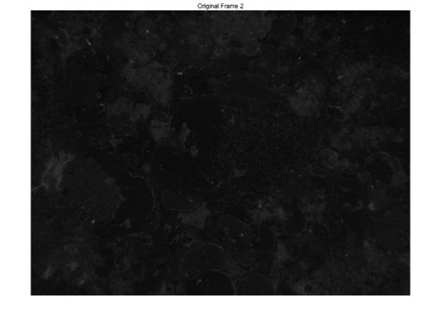
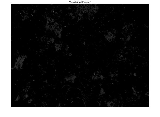
Figure 7: Comparison of the next frame sonar image before and after threshold filtering.

The sonar image after threshold filtering was converted into a point cloud image. Figure 8 is a three-dimensional point cloud image and Figure 9 is a plane point cloud image. Figure 9 shows that the feature points of the point cloud image after filtering are obvious.

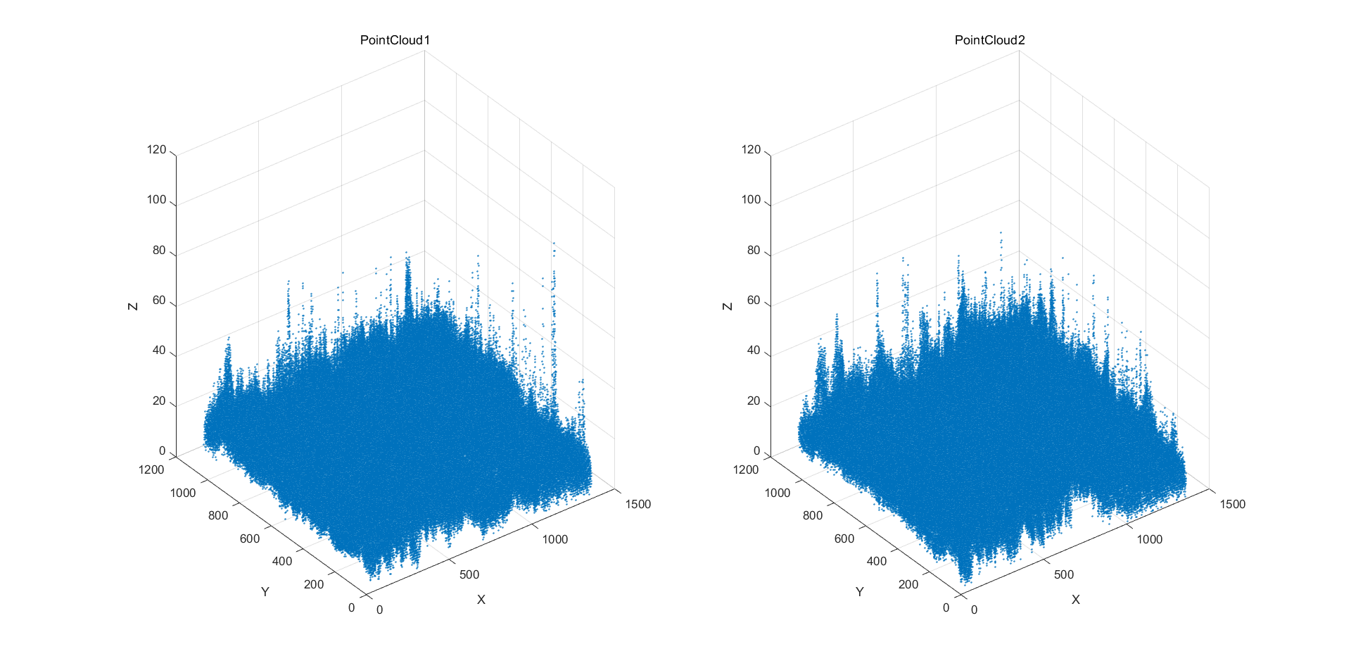
Figure 8: 3D point cloud images of two frames.

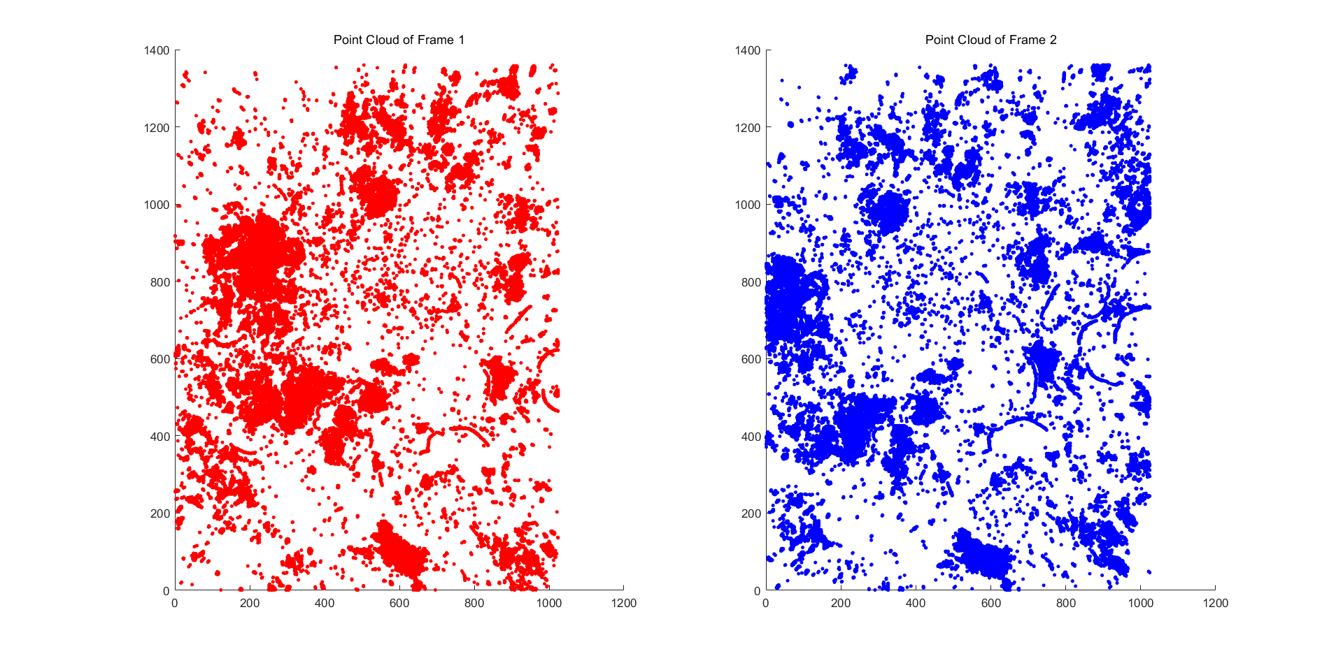
Figure 9: Point cloud images of two frames.

3.2. D Flow Estimation

Visualise the computed 3D flow vectors across the two sonar frames, indicating the pixel motion between them. Figure 10 shows the 3D flow vector of two sonar frames. Based on this, the pixels are classified. Prepare for the follow-up work.

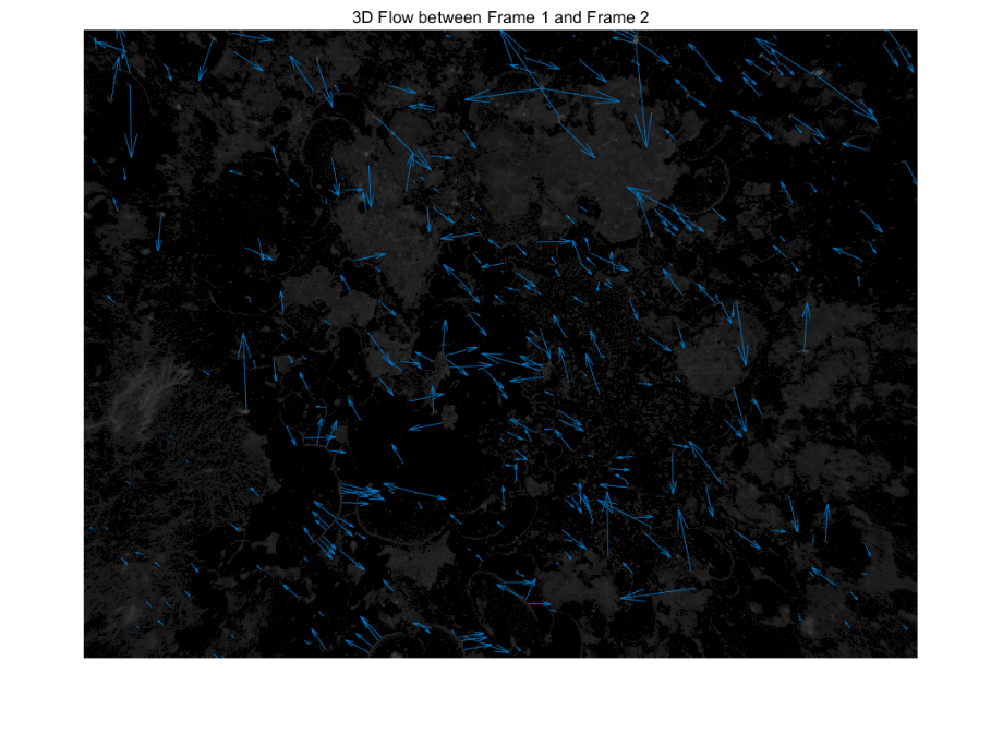
Figure 10: The 3D flow between two frames.

3.3. Feature Point Clustering

Figure 11 shows the movement of different feature points. In the figure, we can see the normal motion trajectory and abnormal motion trajectory. The feature points with abnormal motion trajectories are the dynamic points that need to be eliminated.

The RANSAC algorithm was used to iterate and the dynamic points were detected according to the 3D flow and motion trajectory. The number of iterations of the RANSAC algorithm was set to 5000. After 5000 iterations, we got the interior point, as shown in Figure 12.

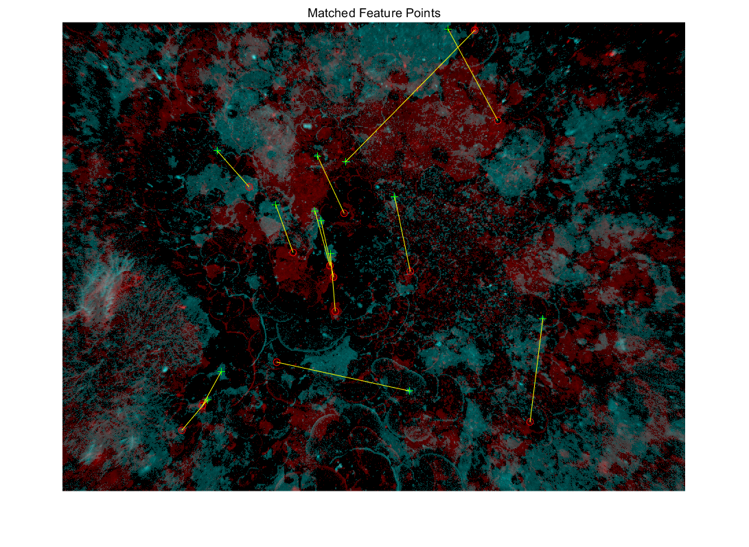
Figure 11: Dynamic point motion trajectory.

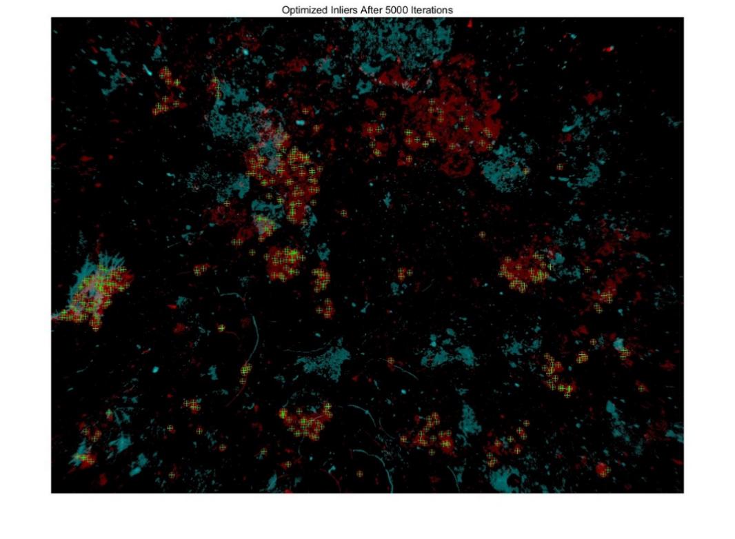
Figure 12: The feature points after elimination.

3.4. Outlier Rejection

The outliers detected by the RANSAC algorithm, that is, dynamic points, were eliminated. The point cloud images before and after elimination are shown in Figure 13.

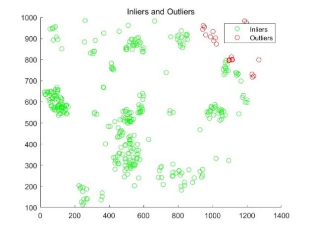
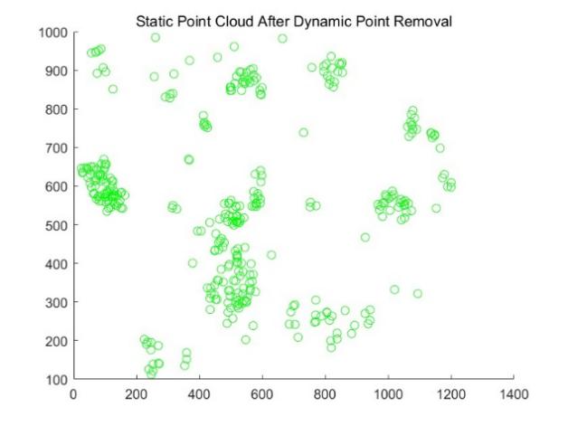
Figure 13: Comparison before and after elimination of outliers.

3.5. Master-Slave AUV Error Curve

The comparison of the position of the main AUV and the slave AUV calculated by the proposed algorithm with the real situation on the ground is shown in the figure. It can be seen that after working for a long time, their trajectory error is very small and because multiple AUVs work at the same time, the task time is greatly shortened and the cumulative error increases with time. The simulation results show the effectiveness of our proposed method.

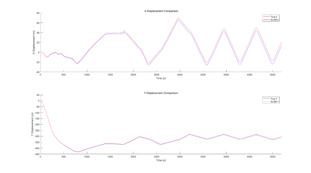
Figure 14: The slam estimation error of the main AUV.

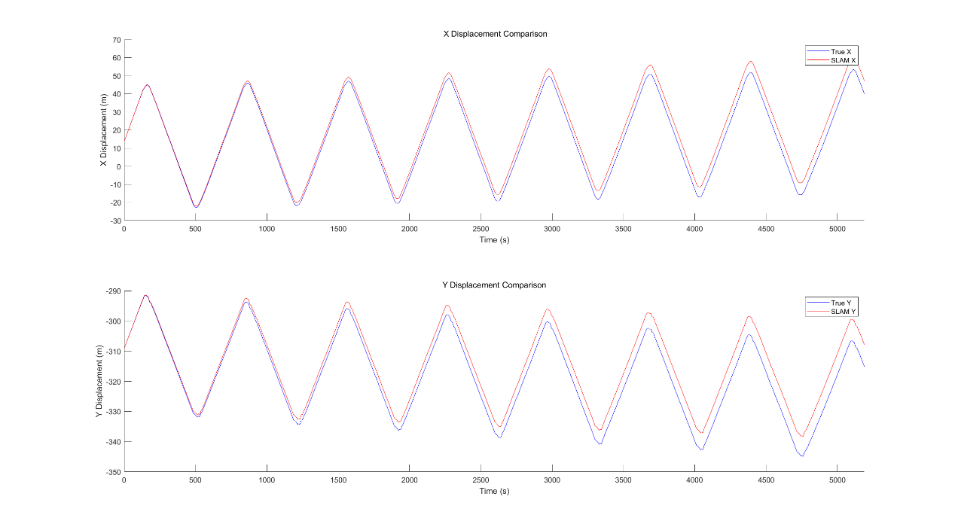
Figure 15: The slam estimation error of the slave AUV1.

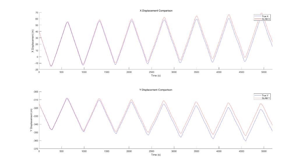
Figure 16: The slam estimation error of the slave AUV2.

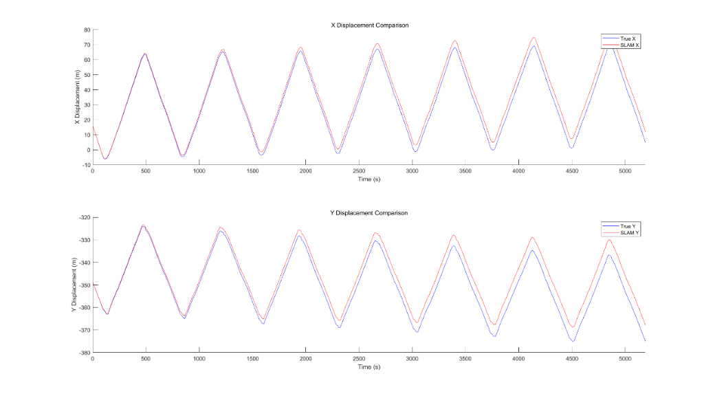
Figure 17: The slam estimation error of the slave AUV3.

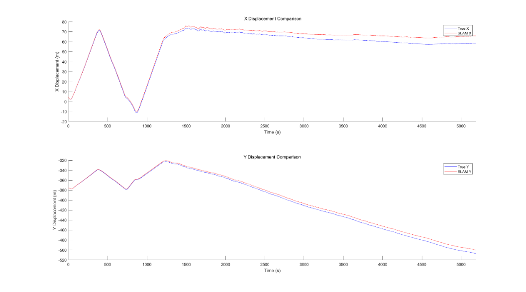
Figure 18: The slam estimation error of the slave AUV4.

4. Discussion

Presently, some problems still remain. For example, the final map fusion can be regarded as an ideal condition. However, in practical engineering, it is difficult to realise the transmission of maps underwater and it is necessary to perform map fusion in the console. In view of these problems, future work must continue to study data transmission methods suitable for underwater.

5. Conclusion

The comparison of the time required for single AUV and multi-AUV SLAM is shown in the following table. It can be seen that multiple AUVs can greatly reduce the time required for the task while ensuring positioning accuracy.

Table 1: Time required for single AUV and multi-AUV SLAM.

6. Summary

This paper proposes a cooperative SLAM algorithm for multi-AUV underwater exploration and mapping. To address the challenges posed by the dynamic environment encountered with multiple AUVs, a RANSAC-based algorithm was introduced to detect and eliminate dynamic points from the sonar data. The proposed approach fuses data from Doppler Velocity Log (DVL), Inertial Measurement Unit (IMU) and Multi-Beam Forward-Looking Sonar (MFLS) sensors.

Subsequently, a Rao-Blackwellised Particle Filter (RBPF)-based SLAM method was employed to mitigate the accumulation of inertial sensor errors and generate accurate occupancy grid maps. The algorithm’s efficiency was evaluated through simulations on the ROS 2 platform, utilising the Scott Reef 25 dataset from the Australian Centre for Field Robotics’ marine robotics group. The results demonstrate improved positioning accuracy and mapping performance, showcasing the potential of the proposed cooperative multi-AUV SLAM approach for efficient underwater exploration and mapping in dynamic environments.

Data Availability Statement

The authors would like to acknowledge the Australian Centre for Field Robotics’ marine robotics group for providing the data.

Funding

This research was funded by Marine Economy Development Special Project of 2024 Guangdong Province, under grant no. GDNRC[2024]43; in part by National Key Research and Development Program, under grant no. 2021YFC3101803; in part by National Natural Science Foundation of China, under grant no. U1906218; in part by Natural Science Foundation of Heilongjiang Province, under grant no. ZD2020D001.

References

[1]. Melo, J. and Matos, A. (2017) Survey on advances on terrain based navigation for autonomous underwater vehicles. Ocean Engineering, 139, 250–264.
[2]. Cheng, C., Wang, C., Yang, D., Liu, W. and Zhang, F. (2022) Underwater localization and mapping based on multi-beam forward looking sonar. Frontiers in Neurorobotics, 15, 189.
[3]. Grisetti, G., Stachniss, C. and Burgard, W. (2007) Improved techniques for grid mapping with Rao-Blackwellized particle filters. IEEE Transactions on Robotics, 23, 34–46.
[4]. Köser, K. and Frese, U. (2020) Challenges in underwater visual navigation and SLAM. AI Technology for Underwater Robots, 96, 125–135.
[5]. Amarasinghe, C., Ratnaweera, A. and Maitripala, S. (2020) Monocular visual slam for underwater navigation in turbid and dynamic environments. American Journal of Mechanical Engineering, 8, 76–87.
[6]. Song, C., Zeng, B., Su, T., Zhang, K. and Cheng, J. (2022) Data association and loop closure in semantic dynamic SLAM using the table retrieval method. Applied Intelligence, 52, 11472–11488.
[7]. Xiao, L., Wang, J., Qiu, X., Rong, Z. and Zou, X. (2019) Dynamic-SLAM: Semantic monocular visual localization and mapping based on deep learning in dynamic environment. Robotics and Autonomous Systems, 117, 1–16.
[8]. Sun, Y., Liu, M. and Meng, M.Q.H. (2017) Improving RGB-D SLAM in dynamic environments: A motion removal approach. Robotics and Autonomous Systems, 89, 110–122.
[9]. Ni, J., Wang, X., Gong, T. and Xie, Y. (2022) An improved adaptive ORB-SLAM method for monocular vision robot under dynamic environments. International Journal of Machine Learning and Cybernetics, 13, 3821–3836
Cite this article
Wu,R. (2024). Cooperative SLAM Algorithm for Multi-AUV Underwater Exploration and Mapping. Applied and Computational Engineering,100,85-99.
Data availability
The datasets used and/or analyzed during the current study will be available from the authors upon reasonable request.
Disclaimer/Publisher's Note
The statements, opinions and data contained in all publications are solely those of the individual author(s) and contributor(s) and not of EWA Publishing and/or the editor(s). EWA Publishing and/or the editor(s) disclaim responsibility for any injury to people or property resulting from any ideas, methods, instructions or products referred to in the content.
About volume
Volume title: Proceedings of the 5th International Conference on Signal Processing and Machine Learning
© 2024 by the author(s). Licensee EWA Publishing, Oxford, UK. This article is an open access article distributed under the terms and
conditions of the Creative Commons Attribution (CC BY) license. Authors who
publish this series agree to the following terms:
1. Authors retain copyright and grant the series right of first publication with the work simultaneously licensed under a Creative Commons
Attribution License that allows others to share the work with an acknowledgment of the work's authorship and initial publication in this
series.
2. Authors are able to enter into separate, additional contractual arrangements for the non-exclusive distribution of the series's published
version of the work (e.g., post it to an institutional repository or publish it in a book), with an acknowledgment of its initial
publication in this series.
3. Authors are permitted and encouraged to post their work online (e.g., in institutional repositories or on their website) prior to and
during the submission process, as it can lead to productive exchanges, as well as earlier and greater citation of published work (See
Open access policy for details).