1. Introduction

In the contemporary era, the energy crisis represents a significant obstacle to the advancement of the automotive industry as a whole[1]. As the vanguard of new energy vehicle innovation, pure electric vehicles will spearhead the development trajectory of China's automotive industry. During the overall design and optimisation of pure electric vehicle products, strategic adjustments to the peak efficiency of the motor and improvements to the body structure can be employed in conjunction with one another to enhance the dynamic performance of the electric vehicles[2]. The utilisation of tools such as AVL CRUISE enables the effective modelling of the dynamic performance and operating conditions of the pure electric vehicles, particularly in urban cycles. Such simulations not only furnish crucial data but also offer invaluable empirical insights for the continuous optimisation of electric vehicles[3]. To illustrate, in the context of a front-drive electric vehicle, this study employed the AVL CRUISE to construct a powertrain model and assess its dynamic performance. The simulation results satisfy the performance and subsequent simulation requirements, with a maximum speed of around 180 km/h, a 100 km acceleration time of 12 seconds, and a maximum hill climbing capacity of 55%. Subsequent research involved a series of variables, including vehicle mass, with the objective of elucidating the relationship between dynamic performance and the various influencing factors. The study employed the data analysis and model fitting techniques to gain a comprehensive understanding of the subject matter and to provide valuable insights and reference points for the optimisation of electric vehicles.

2. Dynamic simulation

2.1. Vehicle Motion Equation

The motor generates the torque and transferred it to the driving wheel by passing through the transmission system. Let \( {F_{t}} \) being the driving force and \( {T_{t}} \) being the torque which is acting on the driving wheel. The equation between \( {F_{t}} \) and \( {T_{t}} \) is

\( {F_{t}}=\frac{{T_{t}}}{r} \)

where \( r \) is the radius of the driving wheel. Considering the aggregate transmission ratio \( i \) of transmission system and the mechanical efficiency \( {η_{T}} \) of the transmission system, the equation is

\( {T_{t}}={T_{tq}}i{η_{T}} \)

where \( {T_{tq}} \) is the output torque of motor. Therefore, the driving force presented by the output torque of motor is

\( {F_{t}}=\frac{{T_{tq}}i{η_{T}}}{r} \)

The resistance must be considered. When vehicles are on the inclined ground, the rolling resistance between ground and wheels is

\( {F_{f}}=mgfcosθ \)

where f is the rolling resistance coefficient and \( θ \) is the angle between inclined ground and horizontal plane.

The air resistance for no wind condition can be calculated by

\( {F_{w}}=\frac{{C_{D}}Au_{a}^{2}}{21.15} \)

where \( {C_{D}} \) is the coefficient of air resistance, A is the windward area. \( {u_{a}} \) is the speed of vehicles, which is calculated by

\( {u_{a}}=0.377\frac{rn}{i} \)

where \( n \) is rpm of motor.

The slope resistance \( {F_{i}} \) can be calculated by

\( {F_{i}}=mgsinθ \)

The acceleration resistance is

\( {F_{j}}=δm\frac{d{u_{a}}}{dt} \)

where \( δ \) is automotive rotating mass conversion factor

Therefore, from the driving equation of electric vehicle

\( {F_{t}}={F_{f}}+{F_{w}}+{F_{i}}+{F_{j}} \)

\( \frac{{T_{tq}}i{η_{T}}}{r}=mgfcosθ+\frac{{C_{D}}Au_{a}^{2}}{21.15}+{F_{i}}+mgsinθ+m\frac{d{u_{a}}}{dt} \)

2.2. Select Pure Vehicle Parameters

The parameters of the pure electric vehicle that is selected in this article and the model of pure electric vehicle that is built by Avl Cruise are given below

Table 1. Driving Parameters and Motor Battery

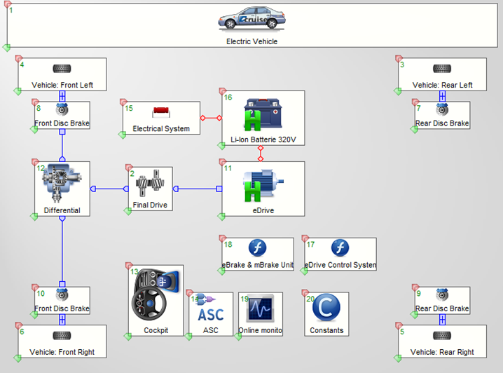
Figure 1. Urban Cycle Simulation of Distance, Velocity and Acceleration pf VehiclesFigure The Pure Electric Vehicle Model

2.3. Simulation results and analysis

To meet the requirements for analyzing real-time simulation of pure electric vehicle performance, it is necessary to select appropriate simulation task environment and vehicle conditions[4]. This process involves implementing simulation with optical step value and acceleration accuracy. The simulation task includes real-time simulation of maximum speed performance in constant drive simulation tasks; real-time simulation of maximum acceleration accuracy performance in full-load acceleration simulation tasks; and simulation of climbing performance in climbing tasks and performance tasks[5].

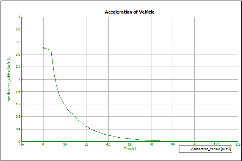
Figure 2. Simulation of acceleration performance

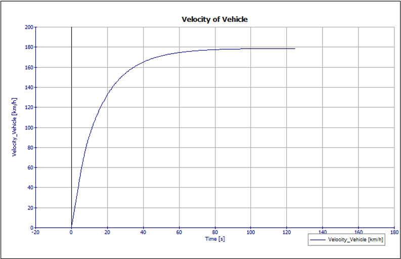
Figure 3. Maximum Speed Acceleration

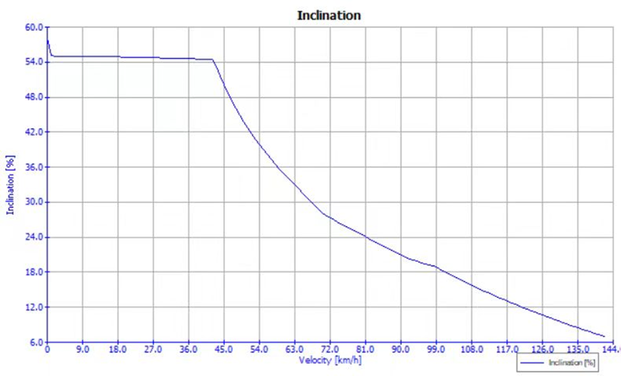
Figure 4. Simulation of acceleration performance

According to Figures 1 and 2, the maximum acceleration of the simulated electric vehicle is about 3 \( {m/s^{2}} \) , and the 100 \( km \) acceleration time is about 12 \( s \) . The acceleration time of the vehicle from standstill to 50 \( km/h \) is about 5 \( s \) , and the static acceleration response time at 50 to 80 \( km \) is about 3.5 \( s \) . According to Figure 2, the maximum speed of the vehicle is approximately 180 \( km/h \) . In terms of Figure 3, the max climb slop is around 57%. The slop remains at approximately 55% in the range of 1 \( km/h \) and 43 \( km/h \) , followed by a continuous decrease to 7% which the velocity raises to 144 \( km/h \) .Therefore, the acceleration performance and maximum speed as well as climb performance of the model meet the design requirements.

3. FTP75 cycle performance simulation and optimization

3.1. FTP75 cycle simulation

The parameters of the selected electric vehicle are still consistent with those above. The simulation model of electric vehicle built is shown in Figure 1:

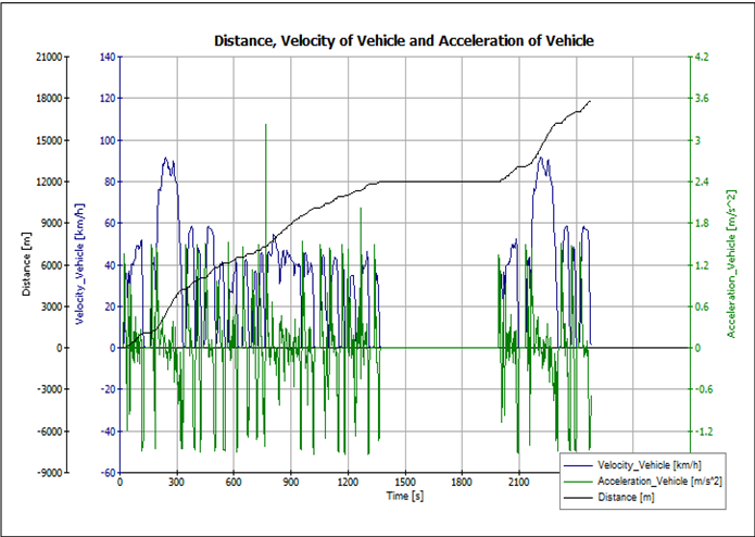
Figure 5. FTP75 Cycle Simulation of Distance, Velocity and Acceleration VehiclesFigure The Pure Electric Vehicle Model

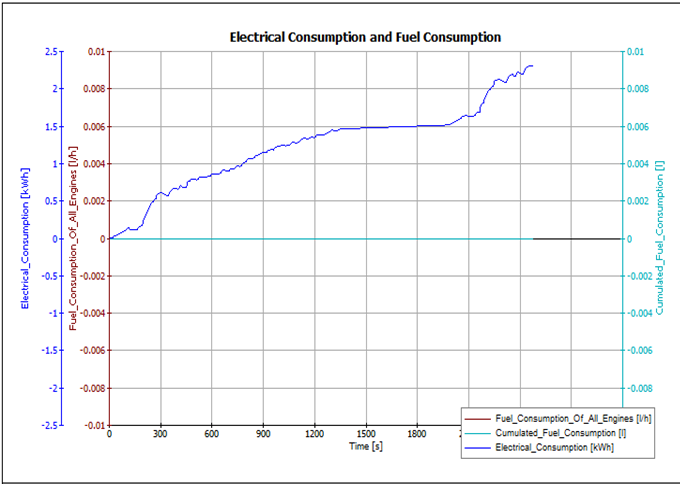
Figure 6. FTP75 Cycle Simulation of Electrical Consumption and Fuel Consumption

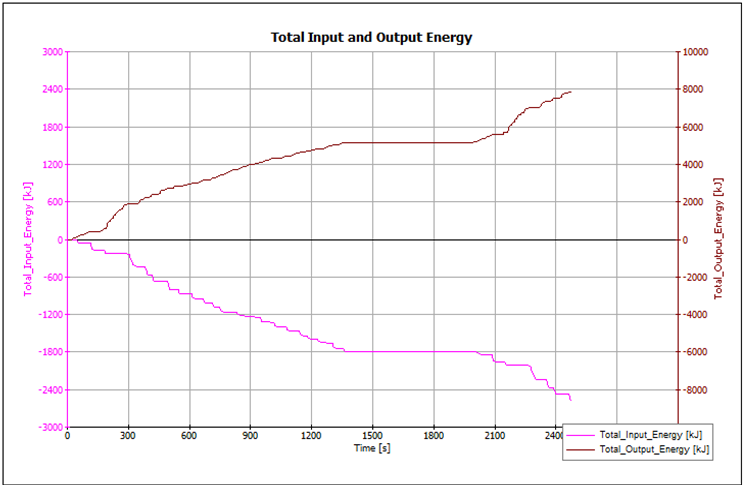
Figure 7. FTP75 Cycle Simulation for Electric Machine eDrive of Total Input and Output Energy

The following presents urban cycle simulation data based on AVL Cruise, with Figures 5, 6, and 7 illustrating the Distance, Velocity, and Acceleration of Vehicles, Electrical Consumption and Fuel Consumption, and Electric Machine eDrive of Total Input and Output respectively (the parameters of the vehicle model remain unchanged, as previously described). According to Figure 6, the Electrical Consumption at the end of the urban cycle is approximately 0.009 \( kWh \) . As shown in Figure 7, the final energy consumption of the electric vehicle is almost 8000 \( kJ \) . To address the energy consumption issues prevalent in most vehicles on the market, the factors affecting vehicle energy consumption under urban cycle conditions will be discussed below.

3.2. Analysis on the influencing factors of energy consumption of pure electric vehicle in city cycle condition

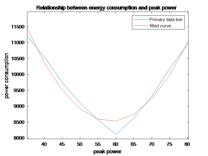
Figure 8. Relationship between energy consumption and peak power

From the figure 8, the energy consumption is obtained by change the peak power value of the motor when simulation in the city cycle condition. According to fitting results, the relationship between the motor power and energy consumption is,

\( E=5{P^{2}}-631P+27004 \)

where it is in the city cycle condition and there is no limitation of velocity. What’s more, in order to reduce the energy waste, the power of the motor should be remained at around 60 kw.

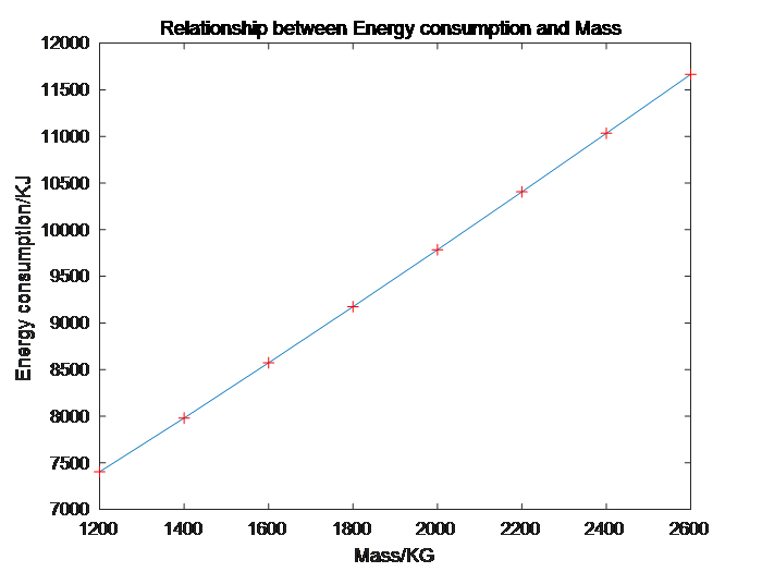
Figure 9. Relationship between energy consumption and Mass

According to figure 9, mass and energy consumption has an approximate linear relevance. Spss is used to conduct correlation analysis based on Pearson coefficient method, and the correlation coefficient obtained is 0.929, indicating a significant correlation. Therefore, the equation of mass and energy consumption is,

\( E=3M+3725 \)

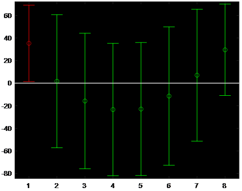
Figure 10. residual plot

In terms of the figure 6, the residual analysis is showed. All the data points are in the confidence interval. As a results, the energy consumption could be decreased each 300 \( kJ \) when the mass is reduced every 100 kg. Thus, the energy use could be reduced by reducing the mass of the vehicle. For example, optimize vehicle chassis design and structure, thereby reducing chassis mass or optimize the structure of the battery and reduce the mass of the battery.

4. Conclusion

In conclusion, this paper presents the development of a simulation model of a pure electric vehicle and its subsequent evaluation of powertrain performance utilising AVL Cruise. The initial evaluation of the model concerned the dynamic performance of the electric vehicle. The simulation results demonstrated that the electric vehicle met the design requirements in terms of top speed, 100 km acceleration time and hill climbing ability, which were 180 km/s, 12 seconds and 55%, respectively. The model also analyses the factors affecting the performance of the pure electric vehicle in the urban cycle. The simulation results demonstrate that the power consumption at the conclusion of the urban cycle is approximately 0.009 kWh, with the final energy consumption of the pure electric vehicle approaching 8000 kJ. Following the adjustment of the parameters and optimisation of the simulation, the results demonstrate a squared-fit relationship between the peak engine power value and the energy consumption. Furthermore, the energy consumption is observed to decrease when the peak engine power value is increased. As the peak engine power increases, so too does the energy consumption. However, when the peak engine power is increased further, the energy consumption is lowest when the engine power is maintained at approximately 60 kW. Thereafter, the energy consumption begins to increase. Concurrently, a linear relationship exists between vehicle mass and energy consumption, whereby energy consumption decreases as vehicle mass decreases. The model offers invaluable data and insights that can be leveraged to optimise electric vehicles, thereby expanding the scope and focus of electric vehicle development.

References

[1]. Yajuan Yang;Han Zhao;Hao Jiang.Drive Train Design and Modeling of a Parallel Diesel Hybrid Electric Bus Based on AVL/Cruise[J].World Electric Vehicle Journal, 2010, 4(1):75.
[2]. Nemes Dániel;Hajdu Sándor.Vehicle Dynamics Modelling of the Mercedes-Benz REFORM 501 LE Urban Bus by Using AVL Cruise Software, 2022:793-798.
[3]. R.Yu. Ilimbetov;V.V. Popov;A.G. Vozmilov.Comparative Analysis of “NGTU – Electro” Electric Car Movement Processes Modeling in MATLAB Simulink and AVL Cruise Software[J].Procedia Engineering, 2015, 129(C):879-885.
[4]. Jianwei Ma.A parameter matching study for power system of electric sweeping vehicle based on AVL CRUISE[J].International Journal of Electric and Hybrid Vehicles, 2020, 12(2).
[5]. Norbert Bagameri;Bogdan Ovidiu Varga;Dan Moldovanu;Aron Csato;Dimitrios Karamousantas.Analysis of Range Extended Hybrid Vehicle with Rotary Internal Combustion Engine Using AVL Cruise, 2018:312-319.
Cite this article
Du,Z. (2024). Based on AVl CRUISE pure electric vehicle simulation and FTP75 circle power consumption factor analysis. Applied and Computational Engineering,114,16-24.
Data availability
The datasets used and/or analyzed during the current study will be available from the authors upon reasonable request.
Disclaimer/Publisher's Note
The statements, opinions and data contained in all publications are solely those of the individual author(s) and contributor(s) and not of EWA Publishing and/or the editor(s). EWA Publishing and/or the editor(s) disclaim responsibility for any injury to people or property resulting from any ideas, methods, instructions or products referred to in the content.
About volume
Volume title: Proceedings of the 2nd International Conference on Machine Learning and Automation
© 2024 by the author(s). Licensee EWA Publishing, Oxford, UK. This article is an open access article distributed under the terms and
conditions of the Creative Commons Attribution (CC BY) license. Authors who
publish this series agree to the following terms:
1. Authors retain copyright and grant the series right of first publication with the work simultaneously licensed under a Creative Commons
Attribution License that allows others to share the work with an acknowledgment of the work's authorship and initial publication in this
series.
2. Authors are able to enter into separate, additional contractual arrangements for the non-exclusive distribution of the series's published
version of the work (e.g., post it to an institutional repository or publish it in a book), with an acknowledgment of its initial
publication in this series.
3. Authors are permitted and encouraged to post their work online (e.g., in institutional repositories or on their website) prior to and
during the submission process, as it can lead to productive exchanges, as well as earlier and greater citation of published work (See
Open access policy for details).