1. Introduction

Time series forecasting [1] is a method that utilizes statistical patterns in historical observational data to predict trends, making it widely applicable in fields such as stock markets, healthcare, and meteorology [2]. However, due to the instability of data collection equipment or other disruptive factors, time series data are often incomplete, which makes it challenging for predictive models to capture data variations and distributional characteristics, thereby affecting forecasting accuracy. Consequently, addressing missing values in time series data is essential for improving the performance of predictive models and holds significant importance.

Traditional methods for handling missing values can generally be divided into deletion methods and imputation methods. The deletion method [3] removes missing samples when their impact on the dataset is minimal. For example, Enders [4] proposed listwise deletion (complete case analysis) for scenarios where data are missing completely at random (MCAR) with a large sample size and minimal missing data, simplifying the process and avoiding spurious data. Deletion approaches typically include right-censoring and interval-censoring. For right-censored data, literature [5] provides a classification support vector machine based on error consistency in a generalized probabilistic measure, applying it to estimate mean, median, quantile, and classification issues for censored data. For interval-censored data, literature [6] introduced a Bayesian nonparametric approach for probability fitting. In the case of left-truncated, right-censored data, literature [7] constructed an empirical estimator for quantile differences and proposed a kernel smoothing estimator for quantile differences. Although these methods are effective in some cases, they can lead to partial data becoming entirely missing, hindering the model’s ability to identify intrinsic features and trends in the data. Imputation methods statistically analyze the dataset and fill in missing values based on certain characteristics (such as mean or median) [8].

Most traditional methods for handling missing data focus on sample inference, Bayesian inference, and likelihood inference [7]. Bayesian and likelihood inference are more commonly applied in practical data. When evaluating long-term project performance with randomly missing data and observational data also missing at random, sample sampling can be used to estimate the dataset’s distribution parameters, ignoring the missing mechanism. For randomly missing data where the parameters of the missing mechanism differ from the dataset distribution parameters, Bayesian inference and likelihood inference can also disregard the missing mechanism. Literature [9] explores non-random missing issues, including non-ignorable non-response and missingness, often referred to as informative missingness.

Recently, with the rapid development of machine learning, these techniques have demonstrated significant advantages in handling missing values. Machine learning methods can extract underlying information and distribution characteristics from data, leading to their widespread application in missing value imputation across various fields. By applying algorithms such as Support Vector Machine (SVM), Random Forest (RF), and Decision Tree (DT), researchers capture the complexity and diversity in the data [10]. A comparative study of RF and neural networks in data imputation showed that RF provides higher accuracy and faster computation for categorical missing data. Deb et al. [11] proposed a Decision Tree-based Stochastic Missing Imputation (DSMI) method, examining imputation rules for missing values. Zhao Lei et al. [12] used well-logging data with SVM for missing data imputation, finding that SVM outperformed regression methods with small sample sizes. Zhang Chan [13] proposed an SVM-based missing value imputation method, which demonstrated higher accuracy and better noise resistance compared to mean imputation and Decision Tree regression methods. Moreover, machine learning techniques allow for considerations of data uncertainty and complexity when imputing missing values. For instance, some methods utilize probabilistic models to evaluate the credibility of imputed values, providing data analysts with additional information. This approach not only provides point estimates for missing values but also offers confidence intervals for the imputed values, which is valuable for data interpretation and further analysis.

Based on the above analysis, we propose an LSTM-based method for handling missing values in time series data. By leveraging the model’s strong spatiotemporal predictive capabilities, we aim to accurately predict missing values to ensure the validity and completeness of the overall time series data.

2. Research Methodology

2.1. Mean Prediction

A common approach for handling missing values is to fill them in based on the mean value of the series with missing values. First, the mean is calculated from the known data:

\( \bar{x}=\frac{1}{n}({x_{1}}+{x_{2}}+{x_{3}}+⋯⋯+{x_{n}}),{x_{1}},{x_{2}},⋯⋯,{x_{n}} represents fixed data \) (2.1)

Then, the calculated mean is directly used to fill in the missing data.

2.2. RNN-Based Methods

For a given sequence \( X=({x_{1}},{x_{2}},{x_{3}},……,{x_{n}})X=({x_{1}},{x_{2}},{x_{3}},……,{x_{n}}) \) , a standard RNN [14] model can generate a hidden layer sequence \( h=({h_{1}},{h_{2}},……,{h_{n}})h=({h_{1}},{h_{2}},……,{h_{n}}) \) and an output sequence \( y=({y_{1}},{y_{2}},……,{y_{n}})y=({y_{1}},{y_{2}},……,{y_{n}}) \) through the iterative calculations shown in Equations (2.2) to (2.3):

\( {h_{t}}={f_{a}}({W_{xh}}{x_{i}}+{W_{hh}}{h_{t-1}}+{b_{h}}){h_{t}}={f_{a}}({W_{xh}}{x_{i}}+{W_{hh}}{h_{t-1}}+{b_{h}}) \) (2.2)

\( {y_{t}}={W_{hy}}{h_{t}}+{b_{y}}{y_{t}}={W_{hy}}{h_{t}}+{b_{y}} \) (2.3)

where \( WW \) represents the weight matrix, \( bb \) the bias vector, and \( {f_{a}}{f_{a}} \) the activation function. The subscript t indicates the time step.

2.3. LSTM

Although RNNs can effectively handle nonlinear time series, they still face two key challenges [15]: (1) due to the vanishing and exploding gradient problems, RNNs are unable to process time series with long-term dependencies; (2) training an RNN model requires a predetermined delay window length, which is often challenging to optimize automatically in real-world applications. This led to the development of the LSTM model. The LSTM replaces the RNN hidden layer cells with LSTM cells, endowing the model with long-term memory capabilities. The most commonly used LSTM cell structure today can be forward-calculated as follows:

\( {i_{t}}=σ({W_{xi}}{x_{i}}+{W_{hi}}{h_{t-1}}+{W_{ci}}{c_{t-1}}+{b_{i}}){i_{t}}=σ({W_{xi}}{x_{i}}+{W_{hi}}{h_{t-1}}+{W_{ci}}{c_{t-1}}+{b_{i}}) \) (2.4)

\( {f_{t}}=σ({W_{xf}}x+{W_{hf}}{h_{t-1}}+{W_{cf}}{c_{t-1}}+{b_{f}}){f_{t}}=σ({W_{xf}}x+{W_{hf}}{h_{t-1}}+{W_{cf}}{c_{t-1}}+{b_{f}}) \) (2.5)

\( {c_{t}}={f_{t}}{c_{t-1}}+{i_{t}}tanh{(}{W_{xc}}{x_{t}}+{W_{hc}}{h_{t-1}}+{b_{c}}){c_{t}}={f_{t}}{c_{t-1}}+{i_{t}}tanh{(}{W_{xc}}{x_{t}}+{W_{hc}}{h_{t-1}}+{b_{c}}) \) (2.6)

\( {ο_{t}}=σ({W_{xo}}+{W_{ho}}{h_{t-1}}+{W_{co}}{c_{t}}+bo){ο_{t}}=σ({W_{xo}}+{W_{ho}}{h_{t-1}}+{W_{co}}{c_{t}}+bo) \) (2.7)

\( {h_{t}}={o_{t}}tanh{(}{c_{i}}){h_{t}}={o_{t}}tanh{(}{c_{i}}) \) (2.8)

where i, f, c, and o represent the input gate, forget gate, cell state, and output gate, respectively. W and b denote the respective weight matrices and bias terms, while σ and tanh represent the sigmoid and hyperbolic tangent activation functions. The LSTM model’s training process utilizes the Back Propagation Through Time (BPTT) algorithm, which is similar in principle to the classical Back Propagation (BP) algorithm. The process generally involves four steps: (1) calculating the output of each LSTM cell based on the forward calculation method; (2) performing backpropagation for each LSTM cell’s error terms, both temporally and across network layers; (3) computing the gradient of each weight based on the error terms; and (4) updating the weights using a gradient-based optimization algorithm.

In the input layer, a continuous segment of the data, \( {X_{0}}=\lbrace {x_{1}},{x_{2}},……{x_{n}}\rbrace {X_{0}}=\lbrace {x_{1}},{x_{2}},……{x_{n}}\rbrace \) , without missing values is divided into the training set \( {X_{tr}}=\lbrace {x_{1}},{x_{2}},……{x_{m}}\rbrace {X_{tr}}=\lbrace {x_{1}},{x_{2}},……{x_{m}}\rbrace \) , the test set \( {X_{te}}=\lbrace {x_{m}}+1,{x_{m}},……{x_{p}}\rbrace {X_{te}}=\lbrace {x_{m}}+1,{x_{m}},……{x_{p}}\rbrace \) , and the validation set \( {X_{ve}}=\lbrace {x_{p+1}},{x_{p+2}},……{x_{n}}\rbrace {X_{ve}}=\lbrace {x_{p+1}},{x_{p+2}},……{x_{n}}\rbrace \) , where \( m \lt p \lt n and m,p,n∈N \) .

Set the sliding window length as L, and divide the normalized training set into multiple windows. The input for each window is \( X=\lbrace {X_{1}},{X_{2}},⋯⋯,{X_{L}}\rbrace {X_{p}}=\lbrace x_{p}^{ \prime },x_{p+1}^{ \prime }.……,x_{m-L+p-1}^{ \prime }\rbrace ,1≤p≤L;p,L∈N{X_{p}}=\lbrace x_{p}^{ \prime },x_{p+1}^{ \prime }.……,x_{m-L+p-1}^{ \prime }\rbrace ,1≤p≤L;p,L∈N \) , and the output is Y \( =\lbrace {Y_{1}},{Y_{2}},⋯⋯,{Y_{L}}\rbrace {Y_{p}}=\lbrace x_{p+1}^{ \prime },x_{p+2}^{ \prime },……,x_{m-l+p}^{ \prime }\rbrace {Y_{p}}=\lbrace x_{p+1}^{ \prime },x_{p+2}^{ \prime },……,x_{m-l+p}^{ \prime }\rbrace \) . The output of the hidden layer is:

\( p=\lbrace {p_{1}},{p_{2}},……{p_{L}}\rbrace p=\lbrace {p_{1}},{p_{2}},……{p_{L}}\rbrace \) (2.9)

\( {p_{p}}=LSTM（{X_{p}},{c_{p-1}},{H_{p-1}}）{p_{p}}=LSTM（{X_{p}},{c_{p-1}},{H_{p-1}}） \) (2.10)

where Cp-1 and Hp-1 are the previous LSTM cell’s state and output, respectively. Assuming the cell state vector size is Sstate, both vectors Cp-1 and Hp-1 have a size of Sstate.

\( loss=\sum _{i=1}^{L(m-L)}\frac{({p_{i}}-{y_{i}}{)^{2}}}{[L(m-L)]}loss=\sum _{i=1}^{L(m-L)}\frac{({p_{i}}-{y_{i}}{)^{2}}}{[L(m-L)]} \) (2.11)

Using the validation set, the mean squared error (MSE) is calculated as follows:

\( MSE=\frac{1}{N}\sum _{n=1}^{N}({\hat{y}_{n}}-{y_{n}}{)^{2}}MSE=\frac{1}{N}\sum _{n=1}^{N}({\hat{y}_{n}}-{y_{n}}{)^{2}} \) (2.12)

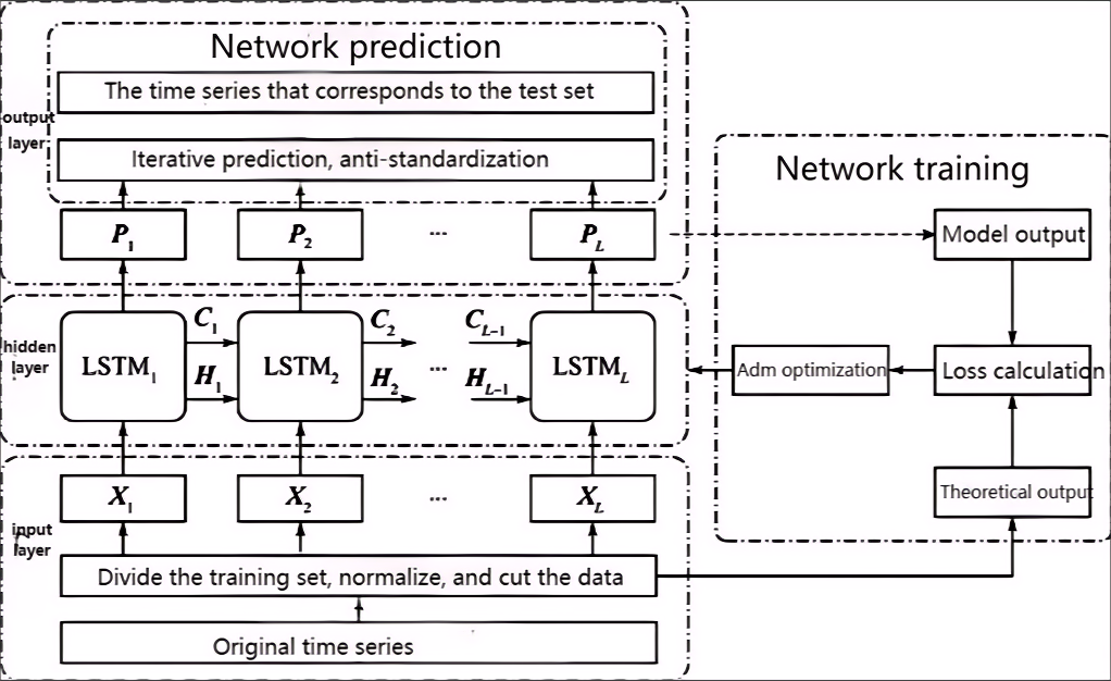
Figure 1. Network Structure

3. Experimental Validation

3.1. Dataset and Preprocessing

The dataset selected for this experiment includes water consumption data from 20 different zones, labeled from flow1 to flow20, all recorded hourly over the same period. The dataset structure consists of multiple columns, where the leftmost column represents time (one data point per hour), and the last column serves as a label, distinguishing different parts of the dataset.

Specifically, the dataset labels are categorized as follows:

Train: This label indicates data used to train the model. The water consumption data in this section is discretely distributed, meaning that each time point’s water usage is given as an independent value, potentially with fluctuations or jumps.

Test1, test2, test3, test4: These labels identify four different test sets, where the water consumption data is provided in a continuous distribution format. This implies that in these test sets, water usage data may show smoother or more continuous variation, lacking the discrete jumps seen in the training set.

It is worth noting that the training set (train) includes not only complete data points but also some missing values. In contrast, the test sets (test1 to test4) display a unique structure, with large sections of blank values (i.e., missing data across multiple consecutive time points).

In this study, we employed a combination of data preprocessing and machine learning models to handle and predict the missing values in the dataset. The specific steps are as follows:

The entire dataset was divided into four subsets, each containing both test and train labels. Initially, we addressed the missing values in the train label by using mean imputation to fill in these gaps. In each subset, features were extracted based on the training set, and a sliding window of length 5 was constructed. To ensure reproducibility, a fixed random seed was used to shuffle the data, creating the training, test, and validation sets.

3.2. LSTM Model Construction and Evaluation

We constructed a Long Short-Term Memory (LSTM) model and evaluated its accuracy by comparing the predictions on the validation set with the actual data, using the Mean Squared Error (MSE) as the evaluation metric. This process allowed us to assess the model’s accuracy in forecasting data.

3.3. Single Feature Prediction

In addition to processing the entire dataset, we conducted an analysis on individual features. We selected a continuous interval without missing values and divided it into training, test, and validation sets. We then created a sliding window and trained the LSTM model. By comparing the test data with the model’s predictions, we calculated the MSE again to evaluate the model’s performance in predicting missing values for individual features.

For the first single feature, we obtained an MSE of 0.401296742814858.

In summary, our experimental results indicate that effective data preprocessing combined with the selection of an appropriate machine learning model can significantly improve the accuracy of missing data predictions in the dataset. Due to its powerful capabilities in time series analysis, the LSTM model proved to be the optimal choice for missing value prediction in this study.

Table 1. Comparison of missing data predication performances

4. Conclusion

This study systematically demonstrates the effectiveness and accuracy of a time series missing data prediction method based on the Long Short-Term Memory (LSTM) model through in-depth analysis and experimental validation. Our approach not only learns from training data with missing values but also efficiently predicts in test sets containing continuous missing segments. By combining mean imputation with a sliding window mechanism, the model fully leverages the intrinsic temporal dependencies in time series data, significantly enhancing prediction accuracy.

Experimental results indicate that our model performs exceptionally across multiple test sets, with low Mean Squared Error (MSE) further affirming its stability and reliability. Additionally, this study explores the model’s predictive capability on individual feature dimensions, demonstrating that the LSTM model is not only suitable for predicting missing values across entire datasets but also excels in single-feature predictions. This finding underscores that the LSTM model is effective for handling both complex, multidimensional data and individual feature missing values with high accuracy.

Compared to previous work, our method shows improvements in the following areas:

Missing Value Imputation Strategy: Traditional methods largely rely on linear interpolation or simple mean imputation, while our approach enhances temporal dependency capture through the introduction of a sliding window mechanism.

Handling of Continuous Missing Segments: Some traditional models experience significant performance degradation with extended missing intervals, whereas our model maintains stable prediction performance even under these conditions.

Single-Feature Prediction Capability: Unlike models requiring multi-feature support, our method demonstrates efficient prediction capability with single-feature data, showcasing its advantages in low-dimensional data scenarios.

Future research can build upon this study to explore more complex deep learning architectures and optimization algorithms, such as incorporating Transformer architectures or attention mechanisms, to further improve prediction accuracy and computational efficiency. Moreover, tailored model optimization strategies for various types of time series data (e.g., non-stationary series) can be developed to expand the application scope of this method.

References

[1]. Wang, X., Wu, J., Liu, C., et al. (2018). Fault Time Series Prediction Based on LSTM Recurrent Neural Network. Journal.
[2]. Wang, G., & Yang, J. (2018). Bidirectional Knowledge and Data-Driven Multigranular Cognitive Computing. Journal of Northwest University (Natural Science Edition), 48(4), 488-500.
[3]. Peugh, J. L., & Enders, C. K. (2004). Missing Data in Educational Research: A Review of Reporting Practices and Suggestions for Improvement. Review of Educational Research, 74, 525-556.
[4]. Enders, C. K. (2010). Applied Missing Data Analysis (p. 7). New York: The Guilford Press.
[5]. Goldberg, Y., & Kosorok, M. R. (2017). Support Vector Regression for Right-Censored Data. Electronic Journal of Statistics, 11(1), 532-569.
[6]. Wu, Y. J., Fang, W. Q., Cheng, L. H., et al. (2018). A Flexible Bayesian Non-Parametric Approach for Fitting the Odds to Case II Interval-Censored Data. Journal of Statistical Computation and Simulation, 88(16), 3132-3150.
[7]. Li, X., & Zhou, Y. (2017). Estimators and Their Asymptotic Properties for Quantile Difference with Left-Truncated and Right-Censored Data. Acta Mathematica Sinica (Chinese Series), 60(3), 451-464.
[8]. Lei, H., Mai, R., Wushouer, et al. (2021). Review of Novelty Detection. Journal of Computer Engineering & Applications, 57(5).
[9]. Fang, F., & Shao, J. (2016). Model Selection with Nonignorable Nonresponse. Biometrika, 103(4), asw039.
[10]. Yu, H. Y., Shen, J., & Xu, M. (2016). Resilient Parallel Similarity-Based Reasoning for Classifying Heterogeneous Medical Cases in MapReduce. Digital Communications & Networks, 2(3), 145-150.
[11]. Deb, R., & Liew, W. C. (2016). Missing Value Imputation for the Analysis of Incomplete Traffic Accident Data. Information Sciences, 339.
[12]. Zhao, L., Li, G., & Ma, X. (2006). Missing Data Completion Method Based on Support Vector Machine. Computer Engineering and Applications, 42(36).
[13]. Zhang, C. (2013). An Algorithm for Missing Value Imputation Based on Support Vector Machine. Computer Applications and Software, 30(5).
[14]. Greff, K., Srivastava, R. K., Koutnik, J., et al. (2016). LSTM: A Search Space Odyssey. IEEE Transactions on Neural Networks & Learning Systems, PP(99), 1-11.
[15]. Ma, X., Tao, Z., Wang, Y., et al. (2015). Long Short-Term Memory Neural Network for Traffic Speed Prediction Using Remote Microwave Sensor Data. Transportation Research Part C: Emerging Technologies, 54, 187-197. https://doi.org/10.1016/j.trc.2015.03.014
Cite this article
Chen,J. (2024). LSTM-based Missing Value Filling Analysis of Time Series. Applied and Computational Engineering,113,122-127.
Data availability
The datasets used and/or analyzed during the current study will be available from the authors upon reasonable request.
Disclaimer/Publisher's Note
The statements, opinions and data contained in all publications are solely those of the individual author(s) and contributor(s) and not of EWA Publishing and/or the editor(s). EWA Publishing and/or the editor(s) disclaim responsibility for any injury to people or property resulting from any ideas, methods, instructions or products referred to in the content.
About volume
Volume title: Proceedings of the 2nd International Conference on Machine Learning and Automation
© 2024 by the author(s). Licensee EWA Publishing, Oxford, UK. This article is an open access article distributed under the terms and
conditions of the Creative Commons Attribution (CC BY) license. Authors who
publish this series agree to the following terms:
1. Authors retain copyright and grant the series right of first publication with the work simultaneously licensed under a Creative Commons
Attribution License that allows others to share the work with an acknowledgment of the work's authorship and initial publication in this
series.
2. Authors are able to enter into separate, additional contractual arrangements for the non-exclusive distribution of the series's published
version of the work (e.g., post it to an institutional repository or publish it in a book), with an acknowledgment of its initial
publication in this series.
3. Authors are permitted and encouraged to post their work online (e.g., in institutional repositories or on their website) prior to and
during the submission process, as it can lead to productive exchanges, as well as earlier and greater citation of published work (See
Open access policy for details).