1. Introduction

Spectrogram With the development of hyperspectral remote sensing technology, new hyperspectral sensors are able to collect continuous images with both spectral and spatial features [1]. Hyperspectral imagery is abundant in characteristics, encompassing both spectral and spatial dimensions. Consequently, these images find extensive applications across various fields such as agriculture, environmental surveillance, urban development, and military reconnaissance [2]. Because hyperspectral images have the attribute of three-dimensional stereo images, the combined spatial and spectral features can be fully utilized for image classification in order to obtain better feature information [3]. However, while the hyperspectral image describes rich feature details, there is also a high degree of correlation between the data, which leads to a large amount of data redundancy [4] and increases the computational complexity. Reducing redundancy in spectral data and extracting combined spatial and temporal features of hyperspectral images have emerged as the foremost objectives in the classification of hyperspectral images [5, 6]. In the field of hyperspectral image classification, traditional methods such as Random Forest (RF) [7] and Support Vector Machine (SVM) [8] often fail to achieve high accuracy in classifying spectral features, and traditional methods often fail to accurately extract spatial and spectral features in hyperspectral images. Moreover, these feature extraction techniques require manual configuration based on prior knowledge. The feature information obtained by setting these parameters is typically limited to distinguishing specific objects, resulting in a lack of flexibility and hindering further enhancement of classification performance.

In contemporary research, classification techniques employing Convolutional Neural Networks (CNNs) have gained widespread application. Nonetheless, prevailing hyperspectral classification approaches predominantly utilize single-branch processing, which inadequately addresses the issue of information redundancy in images. Furthermore, because hyperspectral classification neural networks often have deep depth, the amount of neural network parameters is too large, which leads to slow computation and consumes a large amount of computational resources.

In order to solve the above problems, this paper proposes a new dual-channel CNN (convolutional neural networks) convolutional approach. The method first takes the input hyperspectral image information, extracts the spectral features as well as the spatial features separately, and merges them together after various convolutions to carry out the extracted spectral information. Compared with other 2D/3D-CNN models, the proposed model involves fewer parameters and has a relatively high computation rate, which can achieve higher classification accuracy. The modeling experiments in this paper compare several canonical

The proposed HSIC methodologies demonstrate superior performance in experimental and comparative analyses, surpassing other evaluated techniques. The key contributions of this paper are outlined as follows:

(1) The design of dual- -brunch- Based Spatio- Spectral Integrated network, which adds an attention mechanism to classify hyperspectral images through a dual-branch network.

(2) To ensure spatial consistency in hyperspectral image classification, we integrated both channel and spatial attention mechanisms into a dual-branch network. By aggregating the network's outputs, it derived features that maintain the spatial coherence of the image.

(3) Comparison experiments between this network and other networks are designed. It is concluded that this network has better performance in hyperspectral classification problem.

2. Previous Research

2.1. Conventional categorization techniques

SVM effectively identifies spectral features for high-precision classification by selecting suitable kernel functions and parameters. Huang addressed the issues of multiple covariance in spectral data of organic pollutants and overlapping spectral peaks by developing a method for discriminating organic pollutants in drinking water using UV-vis spectra, based on the successive projection algorithm (SPA) and multiclassification support vector machine (M-SVM). Kaige Yang introduced a novel subspace integration method to optimize subspace retention in the SVM integrated system for hyperspectral false classification. Experiments indicate that this method outperforms random subspace approaches in classification performance. [10].

In hyperspectral imaging, each pixel holds extensive spectral data, and random forests effectively leverage this to build robust classification models, excelling in nonlinear and noisy contexts. Tong, F introduced joint regions that merge fixed-size patches with shape-adaptive hyperpixels for enhanced spatial accuracy. The classification model's RF is substituted with Extreme Random Forest (EF) to mitigate overfitting. Experiments on three HSIs demonstrate that the proposed SSDRF yields commendable classification outcomes, surpassing the patch-based DCDRF.[11]

The K-Nearest Neighbor (KNN) algorithm posits that a sample belongs to the category most represented among its k nearest neighbors in feature space. TU Bing introduces a recursive filtering (RF) method combined with KNN for hyperspectral image classification, calculating Euclidean distances between test and training samples to determine category membership based on the k smallest distances. Huanglei presents a similarity measure using Weighted Spatial-Spectral Distance (WSSD) for KNN, developing a new classification algorithm that leverages hyperspectral image properties. This approach incorporates spatial windows and spectral factors to extract spatial and spectral information, enhancing similarity metrics through spatial nearest-neighbor reconstruction. [12].

2.2. Deep Learning Methods

Due to the limitations of traditional models in classification performance and adaptability, deep learning, particularly CNNs, has advanced hyperspectral image classification by effectively extracting spatial-spectral features. Rujun Chen introduced a method utilizing superpixel segmentation and CNN, integrating 2D segmentation with CNN to enhance classification efficiency [13].S. K. Roy introduced the HybridSN network, integrating 2D segmentation with CNN to enhance classification efficiency. Rujun Chen developed a hyperspectral image classification method utilizing superpixel segmentation and CNN to improve spatial-spectral feature utilization and classification performance. The HybridSN network leverages both 2D and 3D convolutions, employing 3D convolution initially, followed by 2D convolution, and ultimately connecting to classifiers. This approach maximizes spectral-spatial feature extraction while mitigating the complexity associated with exclusive 3D convolution use.[14]. Ben Hamida presents a novel 3D deep learning approach for integrated spectral and spatial data processing. The proposed scheme is assessed through experiments on established hyperspectral datasets, demonstrating superior classification performance compared to existing methods while reducing computational costs. [15]. A deep learning based classification method is proposed which builds high-level features hierarchically in an automated manner [16].Wei X P In order to fully utilize the feature extraction capability of CNN and the discriminative capability of LBP features, a two-channel CNN and LBP combined hyperspectral image classification method is proposed [17].

3. Net structure

3.1. Net structure

In the hyperspectral classification process, it utilize a dual-branch network structure to effectively extract spectral and spatial features from hyperspectral images. Each branch operates independently, and the integration of 1D CNN and 2D CNN optimizes computational efficiency. This paper introduces a dual-branch Spatio-Spectral Integrated Network, comprising a spectral feature extraction branch, a spatial feature extraction branch, classifiers, and a Dropout layer to mitigate overfitting.

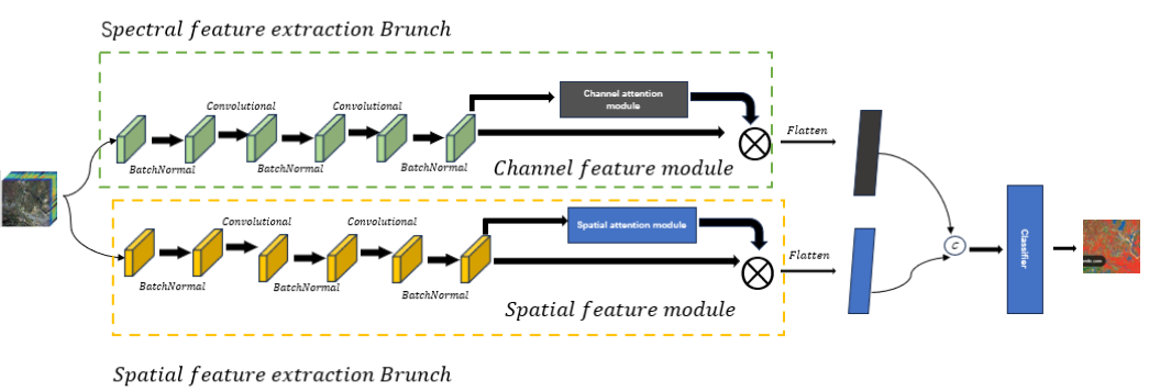
Figure 1: The overall network structure

Figure 1 shows that the network consists of a spectral feature extraction branch, a spatial feature extraction branch, and classifiers, and a Dropout layer is added to the network to mitigate the overfitting problem

In our network, we employ convolutional neural networks to extract spectral and spatial features from hyperspectral images. We define the input matrix size as w, the convolution kernel size as k, the stride as s, and the number of zero-padding layers as p. Consequently, the size of the resulting feature map after convolution is determined as follows:

\( {W^{ \prime }}=\frac{(w+2p-k)}{s}+1 \) (1)

After extracting the feature maps, we flatten each one and splice the maps from both modules to integrate spectral and spatial features, enhancing the model's flexibility and expressiveness. Finally, we apply the Softmax function for classifying the feature classes in the hyperspectral image, as detailed in the following formulas:

\( P(y|x)=\frac{{e^{h(x,{y_{i}})}}}{\sum _{j=1}^{n}{e^{h(x,{y_{i}})}}} \) (2)

3.2. Spectral feature extraction Brunch

In the channel feature extraction module, the input hyperspectral image undergoes three convolutions with kernel sizes of 1x1x32, 1x1x48, and 1x1x120. Each convolution involves sliding the kernel over the input sequence and calculating the inner product at each position. For each position ì, the inner product of the kernel with the subsequence xi+k-1 yields a scalar value. The output sequence element is defined by the activation function, the kernel weights, the input sequence, the bias term, and the kernel size.

\( y[i]= f((\sum _{i=0}^{k-1}{w_{i}}×x[i+j])+b) \) (3)

Each convolutional layer adds Batch Normalization batch regularization to improve the model generalization ability, and adds ReLU, a nonlinear activation function, where the nonlinearity allows the network to learn more complex functions. After convolution, channel attention mechanism is introduced with constant channel dimension and compressed spatial dimension. This module focuses on the channel in hyperspectral will input feature map through two parallel MaxPool layer and AvgPool layer, change the feature map from C*H*W to the size of C*1*1, and then through the MLP module, in which it first compresses the number of channels to the original \( \frac{1}{r} \) times, and then expands to the original number of channels, and then through the ReLU activation function to get the two activated results. These two output results are summed element by element, and the specific expression is as follows:

\( {M_{c}}(F)=σ(MLP(MaxPool(F))+MLP(AvgPool(F))) \) (4)

After getting the result, then through a sigmoid activation function to get the output result of Channel Attention and then multiply this output result by the original figure, change back to the size of C*H*W. Then multiply this output by the original graph and change it back to the size of C*H*W. The network structure of the overall module is shown in Figure2:

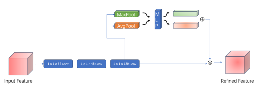
Figure 2: S \( pectral feature extraction Brunch \)

3.3. Spatial feature extraction Brunch

In this module, we first use 2-dimensional convolution to process the spatial information of hyperspectral images with convolution kernel sizes of 10*10*32, 9*9*48, and 8*8*120 respectively, Here if we set the input layer to be \( {W_{in}}×{H_{in}}×{D_{in}} \) ,The number of filters is \( k \) ,The convolution kernel dimension in filters is \( w×h \) ,The slide step is \( s \) ,padding is \( p \) ,output layer is \( {W_{out}}×{H_{out}}×{D_{out}} \) ,The arithmetic relationships are as follows:

\( \begin{cases} \begin{array}{c} {W_{out}}=\frac{{(W_{in}}+2p-w)}{s}+1 \\ {H_{out}}=\frac{{(H_{in}}+2p-w)}{s}+1 \\ {D_{out}}=k \end{array} \end{cases} \) (5)

Subsequently, a spatial attention mechanism is incorporated to maintain the spatial dimension while compressing the channel dimension. The outputs from the convolution operation are derived through max pooling and average pooling, resulting in two feature maps.

Then the two feature maps are spliced and turned into a 1 channel feature map by 7 \( × \) 7 convolution, which is calculated as follows:

\( {M_{c}}(F)=σ({f^{7×7}}([(MaxPool(F));{f^{7×7}}(AvgPool(F))]) \) (6)

The results undergo a sigmoid function to generate the spatial attention feature map, which is then multiplied by the original map to revert to C*H*W dimensions. The network architecture of this module is illustrated in Figure 3.

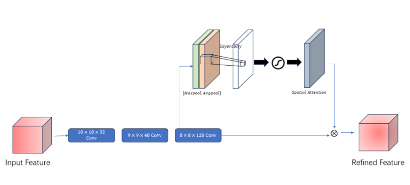
Figure 3: \( Spatial feature extraction Brunch \)

4. Evaluation Process

4.1. Dataset

Three publicly accessible datasets—Indian Pines (IP), Pavia University (PU), and Salinas (SA)—were chosen to evaluate the effectiveness of the proposed algorithm. The IP dataset, captured by NASA's AVIRIS at the Indian Pine Proving Ground in 1992, encompasses 16 distinct classes. It comprises a 145×145 pixel image with a spatial resolution of 20 meters, a spectral resolution of 10 nanometers, and spans a spectral range from 400 to 2,500 nanometers across 224 bands. After excluding 24 bands compromised by noise and water absorption, 200 bands were employed for the experiment. The PU dataset, obtained by the Reflectance Optical System Imaging Spectrometer at the University of Pavia in 2002, includes 9 classes, with an image dimension of 610×340 pixels, a spatial resolution of 1.3 meters, and spectral coverage from 430 to 860 nanometers across 115 bands, ultimately retaining 103 bands after excluding 12 bands affected by noise. The SA dataset, acquired by AVIRIS in 1992 in Salinas Valley, California, comprises 16 classes, with a spatial dimension of 512×217 pixels and a resolution of 3.7 meters. The original image contained 224 bands, but 20 bands affected by water absorption were removed, resulting in 204 bands for analysis.

4.2. Experimental environment and parameter settings

Hardware environment: Windows 11 operating system, computer model Intel(R) Core(TM) i7-14700K @3.60GHz 3.60 GHz+32.0GB, graphics card model NVIDA GeForce RTX 4060ti.

Parameter settings: batch size is set to 128; the number of training rounds (epochs) is set to 200; the ratio of the training set to the test set is 10%; all are randomly selected, and the state of the random number is set to 345; the window size is set to 25; and the learning rate is set to 0.0001.

4.3. Categorized evaluation indicators

The evaluation metrics employed for classification included overall accuracy (OA), average accuracy (AA), and the Kappa coefficient.

OA represents the ratio of the number of correctly categorized pixels in an image to the overall number of pixels, which is calculated as follows:

\( OA=\frac{1}{N}\sum _{1}^{r}{x_{ii}} \) (7)

AA denotes the average value of classification accuracy, which is calculated as follows

\( AA=\frac{(\frac{TP}{TP+FN}+\frac{TN}{FP+TN})}{2} \) (8)

The Kappa coefficient is a measure of consistency that avoids the effects of imbalances in the data categories, and is calculated as follows:

\( {P_{0}}=\frac{\sum _{i=1}^{c}{T_{i}}}{n} \) (9)

\( {P_{e}}=\frac{\sum _{i=1}^{c}{a_{i}}×{b_{i}}}{{n^{2}}} \) (10)

\( Kappe=\frac{{P_{0}}-{P_{e}}}{1-{P_{e}}} \) (11)

4.4. Comparison Experiment

In evaluating the Hyperspectral Image (HSI) classification performance, we employed three key metrics: Overall Accuracy (OA), Average Accuracy (AA), and Kappa Coefficient. OA quantifies the ratio of correctly classified samples to the total sample population, while AA represents the mean accuracy across all classification categories. The Kappa Coefficient serves as a statistical measure that quantifies the agreement between the predicted classification maps and ground-truth references. This paper benchmarked our proposed Spectral-Spatial Deep Belief (SSDB) model against established supervised learning algorithms, including Support Vector Machine (SVM), Random Forest (RF), k-Nearest Neighbors (KNN), three-dimensional Convolutional Neural Network (3D-CNN), and Hybrid Spectral Network (HybridSN). Table1 presents the comparative analysis of these classification methodologies across three standard datasets: Indian Pines (IP), Pavia University (PU), and Salinas (SA).

Table 1: The classification accuracies, expressed as percentages, achieved by both the proposed and state-of-the-art methodologies on a training dataset comprising 10% of the total data.

SSDB outperforms traditional classification methods and shows superior results compared to 3D CNN on the IP dataset, slightly exceeding HybridSN. While its performance on the PU and SA datasets is not as strong as HybridSN, it still achieves high classification accuracy. Additionally, SSDB's training data volume is reduced to 3,393,409 from HybridSN's 5,122,176, resulting in a more lightweight network.

The subsequent illustration presents the outcomes of various classification algorithms applied to the categorized IP dataset depicted in Figure 4.

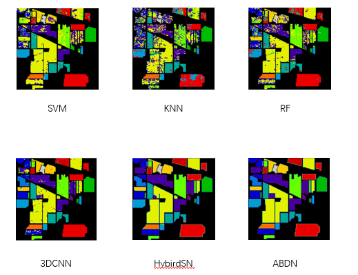
Figure 4: The result of IP

4.5. Ablation Experiment

To assess the efficacy of our proposed network and attention mechanism, we conduct a comparative analysis between the single branch network and the network integrated with the CBAM attention mechanism. The findings are presented in Table 2 below:

Table 2: Compare the accuracy of different network structures and attention mechanisms

The analysis reveals that the classification accuracy of the single-branch network is lower than that of the two-branch network, irrespective of the presence of the attention mechanism. Additionally, the two-branch network incorporating CBAM does not surpass SSDB, indicating that our attention mechanism is more proficient in hyperspectral classification.

4.6. Convergence experiment

The proposed method is applied to IP, SA, and UP datasets, with results analyzed. Loss curves during training are presented in Figure 5. The IP dataset converges after approximately 50 epochs, while the SA and UP datasets, being easier to categorize, converge after about 30 epochs. A lower loss value indicates that the model's predictions are closer to the true values.

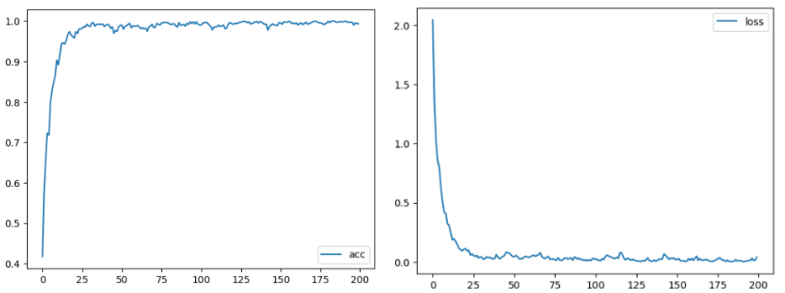
Figure 5: The accuracy and loss on IP dataset

5. Conclusion

In response to the challenges of insufficient feature extraction and overlapping fine details in hyperspectral image data, I introduce a dual-channel hybrid convolutional classification method incorporating an attention mechanism. This model leverages dual branches to comprehensively analyze spatial and spectral information, optimizing feature extraction while minimizing redundancy. The attention mechanism assigns weights to spectral and spatial dimensions to enhance feature differentiation, thereby improving the distinction between background and target, and producing classification results through a fully connected layer. This method effectively harnesses the full spectrum of hyperspectral data features and enhances model generalization. Experimental findings demonstrate that the dual-branch neural network surpasses single-branch models, validating its feasibility and robustness. Nonetheless, further investigation is required to extract deeper spectral and spatial features, refine network parameters, reduce computational complexity, and integrate advanced techniques such as band selection and data augmentation to advance hyperspectral image classification.

References

[1]. ZHANG B. Hyperspectral image processing and information extraction[J]. Journal of Remote Sensing, 2016, 20(5): 1062 1090.
[2]. ZHANG C M, MUYK,YANTY, et al. Overview of hyper spectral remote sensing technology[J]. Spacecraft Recovery & Remote Sensing, 2018, 39(3): 104-114.
[3]. ZHAO W Z, DU S H. Spectral-spatial feature extraction for hyperspectral image classification: a dimension reduction and deep learning approach[J]. IEEE Transactions on Geoscience and Remote Sensing, 2016, 54(8): 4544-4554.
[4]. LIU Y F, LI X R, FENG Y M, et al. Representativeness and redundancy-based band selection for hyperspectral image classification[J]. International Journal of Remote Sensing, 2021, 42(9): 3534-3562.
[5]. SHE H L, XIE S J, ZOU J J. 3D-CNN with standard score dimensionality reduction for hyperspectral remote sensing images classification[J]. Computer Engineering and Appli cations, 2021, 57(4): 169-175.
[6]. YU CY, HAN R, SONG M P,et al.Asimplified 2D-3D CNN architecture for hyperspectral image classification based on spatial-spectral fusion[J]. IEEE Journal of Selected Topics in Applied Earth Observations and Remote Sensing, 2020, 13: 2485-2501.
[7]. Breiman L. Random Forests[J]. Machine Learning, 2001, 45(1):5-32
[8]. M. A. Hearst, S. T. Dumais, E. Osuna, J. Platt and B. Scholkopf, "Support vector machines," in IEEE Intelligent Systems and their Applications, vol. 13, no. 4, pp. 18-28, July-Aug. 1998, doi: 10.1109/5254.708428.
[9]. Cover, Thomas M. and Peter E. Hart. “Nearest neighbor pattern classification.” IEEE Trans. Inf. Theory 13 (1967): 21-27.
[10]. HUANG Ping-jie, LI Yu-han, YU Qiao-jun, WANG Ke, YIN Hang, HOU Di-bo, ZHANG Guang-xin. Classification of Organic Contaminants in Water Distribution Systems Developed by SPA and Multi-Classification SVM Using UV-Vis Spectroscopy[J]. Spectroscopy and Spectral Analysis, 2020,40(7): 2267-2272.
[11]. Tong, F.; Tong, H.; Jiang, J.; Zhang, Y. Multiscale Union Regions Adaptive Sparse Representation for Hyperspectral Image Classification. Remote Sens. 2017, 9, 872.
[12]. HUANG Hong, ZHENG Xin-lei. Hyperspectral image classification with combination of weighted spatial-spectral and KNN[J]. Optics and Precision Engineering, 2016, 24(4): 873
[13]. Rujun Chen, Yunwei Pu, Fengzhen Wu, Yuceng Liu, Qi Li. Hyperspectral Image Classification Based on Hyperpixel Segmentation and Convolutional Neural Network[J]. Laser & Optoelectronics Progress, 2023, 60(16): 1610010
[14]. S. K. Roy, G. Krishna, S. R. Dubey and B. B. Chaudhuri, "HybridSN: Exploring 3-D–2-D CNN Feature Hierarchy for Hyperspectral Image Classification," in IEEE Geoscience and Remote Sensing Letters, vol. 17, no. 2, pp. 277-281, Feb. 2020,
[15]. A. Ben Hamida, A. Benoit, P. Lambert, and C. Ben Amar, “3-d deep learning approach for remote sensing image classification,” IEEE Transactions on geoscience and remote sensing, vol. 56, no. 8, pp. 4420 4434, 2018.
[16]. K. Makantasis, K. Karantzalos, A. Doulamis, and N. Doulamis, “Deep supervised learning for hyperspectral data classification through convo lutional neural networks,” in IEEE International Geoscience and Remote Sensing Symposium (IGARSS). IEEE, 2015, pp. 4959–4962.
[17]. Wei X P,Yu X C,Zhang P Q,Zhi L and Yang F. 2020. CNN with local binary patterns for hyperspectral images classification. Journal of Remote Sensing(Chinese),24(8): 1000-1009
Cite this article
Zhao,X. (2024). Joint Spatial-Spectral Convolutional Neural Network Enhanced with Attention Mechanism for Optimized Hyperspectral Image Classification. Applied and Computational Engineering,115,117-125.
Data availability
The datasets used and/or analyzed during the current study will be available from the authors upon reasonable request.
Disclaimer/Publisher's Note
The statements, opinions and data contained in all publications are solely those of the individual author(s) and contributor(s) and not of EWA Publishing and/or the editor(s). EWA Publishing and/or the editor(s) disclaim responsibility for any injury to people or property resulting from any ideas, methods, instructions or products referred to in the content.
About volume
Volume title: Proceedings of the 5th International Conference on Signal Processing and Machine Learning
© 2024 by the author(s). Licensee EWA Publishing, Oxford, UK. This article is an open access article distributed under the terms and
conditions of the Creative Commons Attribution (CC BY) license. Authors who
publish this series agree to the following terms:
1. Authors retain copyright and grant the series right of first publication with the work simultaneously licensed under a Creative Commons
Attribution License that allows others to share the work with an acknowledgment of the work's authorship and initial publication in this
series.
2. Authors are able to enter into separate, additional contractual arrangements for the non-exclusive distribution of the series's published
version of the work (e.g., post it to an institutional repository or publish it in a book), with an acknowledgment of its initial
publication in this series.
3. Authors are permitted and encouraged to post their work online (e.g., in institutional repositories or on their website) prior to and
during the submission process, as it can lead to productive exchanges, as well as earlier and greater citation of published work (See
Open access policy for details).