


1. Introduction
After the first introduction of Dynamic Time Warping (DTW) in speech recognition[1], machine learning has been using it for its various problems[2-4]. Several review articles[5,6] highlighted the potential of DTW for time series comparison. However, there was a main barrier to using DTW, computational complexity. The time complexity, \(O(NM)\) , provides an approximation of the work required for an algorithm based on the input sizes, \(N\) and \(M\) . Numerous algorithmic strategies to reduce the complexity of DTW have been published however they didn't solve DTW problems exactly[7,8]. \iffalse After the first introduction of Dynamic Time Warping (DTW) in speech recognition[1], it has been proposed as a solution for various machine learning problems[2-4] Several review articles[5,6] highlighted the potential of DTW for time series comparison. However, there was a main barrier to use DTW, computational complexity. The time complexity is in general \(O(NM)\) , where \(N\) and \(M\) are the lengths of the time series. Many algorithmic approaches to reduce the complexity of DTW have been published however they didn?t apply specific problems[7,8]. \fi \iffalse DTW was first introduced in speech recognition [1], and has been applied to a wide range of machine learning problems such as handwriting recognition [2], fingerprint verification [3], classification of motor activities [4] \iffalse [4,9,10] \fi and others. DTW is often viewed as one of the best methods for time series comparison in data mining as discussed in several review articles [5,6]. However, computational complexity has been a barrier to the use of DTW. The time complexity is in general \(O(NM)\) , where \(N\) and \(M\) are the lengths of the time series. There are many algorithmic approaches to reducing the complexity of DTW for general time series which are not tied to specific problems. The interested reader should refer to [7,8]. One common approach is to add a global constraint on slope [11] or width [1] along the diagonal of the warping path domain. Another approach involves multi-resolution approximation [12]. This latter strategy improves the time complexity to \(O(N+M)\) . However, these modifications of DTW can yield solutions which are far from the exact DTW solution. \fi \iffalse One approach to reducing this complexity is to add a global constraint on slope[11] or width[1] along the diagonal of the permissible warping path domain. The complexity can also be reduced by pruning cells of computation whose distances are larger than an upper bound of DTW distance[13]. The so-called PrunedDTW was based on the idea that the distances around the optimal warping path are relatively low but cells distant from the optimal path often have higher distances. It was reported to reduce the time complexity by two on average. Another approach involves a multi-resolution approximation of the time series [12]. Their strategy is to recursively project an optimal warping path computed at a coarse resolution level to the next higher resolution level and then to refine the projected path. This method improves the time complexity to \(O(N)\) . However, none of the above speed enhancements of DTW provably achieve the exact unconstrained solution except for PrunedDTW. In fact, these methods can yield solutions which are quite far from optimal[14]. \fi One of the real-life cases in sparse time series is managing zero values such as periods of silence in speech, inactivity or lack of food intake[15], or periods when house appliances are not running[16]. \iffalse They have been ignored as missing data but\fi They are not missing data but explain the sparse characteristics of the source. \iffalse Recent efforts for complexity reduction in DTW focused on the type of sparsity[8,14,17,18]. \fi To mitigate the challenges when using DTW for such sources, Sparse Dynamic Time Warping (SDTW)[14], Binary Sparse Dynamic Time Warping (BSDTW)[18], Constrained Sparse Dynamic Time Warping (CSDTW)[7], and Constrained Binary sparse Dynamic Time Warping (CBSDTW)[19] were developed and analyzed to speed up the DTW. The new algorithms were equivalent to DTW but had their computational complexities reduced by the sparsity ratio, \(s\) or \(s^2\) (BSDTW, CBSDTW), where \(s\) was defined as the arithmetic mean of the proportion of non-zero values in the data. Also, Fast Sparse Dynamic Warping (FSDTW)[8] and AWarp[17] were developed and analyzed for further speed improvement by the order of \(s^2\) at the expense of accuracy. \iffalse One of the real-life cases in sparse time series is managing zero values such as quiet periods in speech, lack of physical activity or food intake[15], or absence of power usage by appliances[16]. They have been ignored as missing data but they are informative when explaining the characteristics of the source. Recent efforts for complexity reduction in DTW focused on the type of sparsity[8,14,17,18]. \fi \iffalse An important case of sparse time series is one where the data takes zero value at many epochs (when we refer to sparsity in the sequel it is of this type). These zero values are not missing data, but rather are informative and characteristic of their source. For example, zero data arises from quiet periods in speech, lack of physical activity or food intake [15], or absence of power usage by appliances [16]. There has only recently been work on complexity reduction for DTW which specifically takes into account this type of sparsity [8,14,17,18]. \iffalse The binary DTW problem has also received attention from practitioners[18,20,21]. For example, several of the CASAS human activity data sets[22] that have been examined in the context of DTW consist of binary data points (e.g., sensor data indicating when a door is open/closed)[17,23].\fi \fi \iffalse To mitigate the challenges when using DTW, Sparse Dynamic Time Warping (SDTW)[14], Binary Sparse Dynamic Time Warping (BSDTW)[18], Constrained Sparse Dynamic Time Warping (CSDTW)[7], and Constrained Binary sparse Dynamic Time Warping (CBSDTW)[19] were developed to improve the speed of the DTW. The new algorithms were equivalent to DTW but have their computational complexities reduced by the sparsity ratio \(s\) that is defined as the arithmetic mean of the fraction of non-zeros in the two time series. Also, Fast Sparse Dynamic Warping (FSDTW)[8] and AWarp[17] were developed for further speed improvement at the expense of accuracy. \fi \iffalse Sparse dynamic time warping (SDTW) [14] was developed for real-valued time series to exploit such sparsity. SDTW is equivalent to DTW, i.e., it yields the exact DTW distance (and if desired the corresponding warping paths), and the time complexity of SDTW is about \(2s\) times the complexity of DTW, where the sparsity ratio \(s\) is defined as the arithmetic mean of the fraction of non-zeros in the two time series. Binary sparse dynamic time warping (BSDTW) [18] was then developed for comparing binary-valued (1 or 0) time series. BSDTW is equivalent to DTW when restricted to binary values, and the time complexity of BSDTW is about \(2s^{2}\) times the complexity of DTW. \iffalse [21] proposed an algorithm to do DTW in linear time for binary data. \fi AWarp [17] was also developed to compare real-valued time series to exploit sparsity. It's time complexity is about \(4s^{2}\) times the complexity of DTW, and hence is theoretically faster than SDTW for sparse time series. However, AWarp is not in general equivalent to DTW, although it produces impressive results in some applications where the exact DTW solution is not required. \iffalse It is also argued that AWarp is equivalent to DTW for the binary-valued time series. \fi Then, fast sparse dynamic time warping (FSDTW) [8] was developed for general-valued time series to exploit sparsity. FSDTW is a fast and very accurate approximation to DTW based on an simplification of the SDTW. The time complexity of FSDTW is upper bounded by about 6s \(^{2}\) times the complexity of DTW. Hence comparing the worst cases, FSDTW is about 1.5 times slower than AWarp. But It has been shown that for a wide range of examples FSDTW provides similar time complexity and much more accurate approximation to DTW for sparse time series. In fact, the relative error of FSDTW (relative to DTW) is typically \(\sim10^{-4},\) and is several orders of magnitude less than the relative error of AWarp. In addition, constrained sparse dynamic time warping (CSDTW) [7] was developed for the constrained case where the width is limited along the diagonal of the permissible path domain. CSDTW is exactly equivalent to constrained DTW(CDTW) and its time complexity is about \(2s\) times the complexity of CDTW. It turns out that CSDTW updates the data at the intersection of the feasible set that satisfies the constraint and the boundary of certain rectangles determined by the nonsparse time indices, as opposed to the intersection of the feasible set and the indices themselves in DTW. Then, constrained binary sparse dynamic time warping (CBSDTW) [19] was developed for the binary time series and the constrained permissible warping paths. CBSDTW is exactly equivalent to CDTW and its time complexity is about \(3s^2\) times the complexity of CDTW. It turns out that CBSDTW updates the data at the end points of the intersection of the feasible set that satisfies the constraint and the boundary of certain rectangles determined by the nonsparse time indices. \fi \iffalse It is important to note that CSDTW updates the data at the subset of the region where SDTW updates them by taking the intersection with the feasible set. \fi The current study focuses on the faster approximation of CSDTW, Fast Constrained Sparse Dynamic Time Warping (FCSDTW). The time complexity of FCSDTW is upper bounded by about \(6s^2\) times the complexity of CDTW. Even though FCSDTW is slightly slower than constrained AWarp (CAWarp) when comparing worst cases, a wide range of examples of FCSDTW is needed to provide better complexity and a more accurate estimation of CDTW. The relative error of FCSDTW (relative to CDTW) is typically \(\sim10^{-4}\) , and is at least ten-thousandths that of CAWarp. Providing the most rigorous analysis, this study should be a core background for further reduction of time complexity. \iffalse This paper focuses on the faster approximation of CSDTW, Fast Constrained Sparse Dynamic Time Warping (FCSDTW). The time complexity of FCSDTW is upper bounded by about \(6s^2\) times the complexity of CDTW. Even though FCSDTW is about 1.5 times slower than constrained AWarp (CAWarp) when comparing worst cases, a wide range of examples of FCSDTW is needed to provide better complexity and a more accurate approximation to CDTW. The relative error of FCSDTW (relative to CDTW) is typically \(\sim10^{-4}\) , and is at most ten-thousandths times that of CAWarp. Providing the most rigorous analysis, this study should be a core background for further reduction of time complexity. \fi \iffalse Hence comparing the worst cases, FCSDTW is about 1.5 times slower than constrained AWarp (CAWarp). But a wide range of examples of FCSDTW is needed to provide similar time complexity and a much more accurate approximation to CDTW for sparse time series. The relative error of FCSDTW (relative to CDTW) is typically \(\sim10^{-4},\) and is several orders of magnitude less than the relative error of CAWarp. Providing the most rigorous analysis, this study should be a core background for further reduction of time complexity.\fi \iffalse This paper focuses on the development and analysis of a fast approximate algorithm of CDTW based on the CSDTW framework. We call this constrained fast sparse dynamic time warping (FCSDTW). The time complexity of FCSDTW is upper bounded by about 6s \(^{2}\) times the complexity of CDTW. Hence comparing worst cases, FCSDTW is about 1.5 times slower than constrained AWarp (CAWarp). But we shall show that for a wide range of examples FCSDTW provides similar time complexity and much more accurate approximation to CDTW for sparse time series. In fact, the relative error of FCSDTW (relative to CDTW) is typically \(\sim10^{-4},\) and is several orders of magnitude less than the relative error of CAWarp. \iffalse It turns out that FCSDTW updates the data at the end points of the intersection of the feasible set that satisfies the constraint and the boundary of certain rectangles determined by the nonsparse time indices. \fi There are no comparable approaches and rigorous analysis for the exact solution to the constrained problem for this kind of sparse data. Furthermore, this study provides a benchmark and also background to potentially understand how such sparsity might be exploited by approximation of the time series, for further complexity reduction. \fi The review of DTW from the perspective of dynamic programming is not included. The interested reader should refer to the previous publications[7,8]. Section 2 presents the principles of FCSDTW and its reduction of complexity compared to CDTW. Section 3 has a description of the FCSDTW algorithm. Finally, the last section demonstrates the efficiency of FCSDTW with some numerical analysis. \iffalse The review of DTW from the dynamic programming perspective is omitted and the interested reader should refer to the previous publications[7,8]. Section 2 provides the principles of FCSDTW and its complexity reduction compared to CSDTW. Section 3 includes a description of the FCSDTW algorithm. Finally, the last section demonstrates the efficiency of FCSDTW with some numerical analysis. \fi \iffalse Section 2 provides the principles underlying FCSDTW and its complexity reduction while comparing it against CSDTW. Section 3 explicitly describes the FCSDTW algorithm. Finally, the last section presents some numerical analysis to demonstrate the efficiency of FCSDTW.\fi \iffalse The review of DTW from the dynamic programming perspective is omitted and the interested reader should refer to the previous publications[7,8]. Section [???] provides the principles underlying FCSDTW and its complexity reduction while comparing against CSDTW. Section [???] explicitly describes the FCSDTW algorithm. Finally, the last section presents some numerical analysis to demonstrate the efficiency of FCSDTW. \fi \iffalse
2. Review of DTW
DTW originated as a dynamic programming algorithm to compare time series in the presence of timing differences for spoken word recognition [1]. In order to describe the timing differences, consider two time series \(X=(x_{1},x_{2},\cdots,x_{M})\) and \(Y=(y_{1},y_{2},\cdots,y_{N})\) . The timing differences between them can be associated with a sequence of points \(F=(c(1),c(2),\cdots,c(k),\cdots,c(K))\) , where \(c(k)=(m(k),n(k))\) . This sequence realizes a mapping from the time indices of \(X\) onto those of \(Y\) . It is called a warping function. The measure of difference between \(x_{m}\) and \(y_{n}\) is usually given as \(d(c)=d(m,n)=|x_{m}-y_{n}|^{p}\) , where \(0\lt p\lt \infty\) (Euclidean \(p\) -norm). For \(p=0\) , \(d(m,n)=1\) if \(x_{m}\not=y_{n}\) and zero otherwise. \(d(m,n)\) is called the local distance. The minimum of the weighted summation of local distances over all warping functions \(F\) is \(D(X,Y)=\frac{1}{\sum_{k=1}^{K}w(k)}\min_{F}[\sum_{k=1}^{K}d(c(k))w(k)]\) where \(w(k)\) is a nonnegative weighting coefficient. \(D(X,Y)\) is the DTW distance and provides a measure of the difference between \(X\) and \(Y\) after alignment. Restrictions on the warping function \(F\) (or points \(c(k)=(m(k),n(k))\) are usually given as follows. 1) Monotonic conditions: \(m(k-1)\leq m(k)\) and \(n(k-1)\leq n(k)\) . 2) Continuity conditions: \(m(k)-m(k-1)\leq1\) and \(n(k)-n(k-1)\leq1\) . 3) Boundary conditions: \(m(1)=1,n(1)=1\) and \(m(K)=M,n(K)=N\) . Determining the distance \(D(X,Y)\) \iffalse given by Eq. [???]\fi is a problem to which the well-known dynamic programming principle can be applied. \iffalse The basic algorithm is given in the following under the above restrictions on the warping function. Initial condition:
Dynamic Programming equation:
Time-normalized distance:
\(g(k)\) is called the accumulated distance. The algorithm Eq. [???]-[???] can be simplified under the above restrictions on the warping function. \fi Let \(w_{d}\) , \(w_{v}\) , and \(w_{h}\) represent the weights for each diagonal, vertical, and horizontal step. Typically, the weight of the diagonal steps is larger than those of the other steps, because the diagonal step can be regarded as the combination of the vertical step and the horizontal step. Then, the algorithm is given as follows. Its initial condition is given as \(g(1,1)=d(1,1)w_{d}\) . DP-equation can be written as \(g(m,n)=\min[g(m,n-1)+d(m,n)w_{v}, g(m-1,n-1)+d(m,n)w_{d}, g(m-1,n)+d(m,n)w_{h}]\) . Finally, Time-normalized distance is computed as \(D(X,Y)=\frac{1}{\sum w(k)}g(M,N)\) . \(g(m,n)\) is called the accumulated distance and \(\{g(m,n)\) : \(1\leq m\leq M\) , \(1\leq n\leq N\}\) is called the accumulated distance matrix. \iffalse Initial Condition:
DP-equation:
g(m-1,n-1)+d(m,n)w_{d}
g(m-1,n)+d(m,n)w_{h} \end{array}] \end{equation}
Time-normalized distance:
\fi \fi
3. Principles Underlying FCSDTW
This section starts with some notation and review of CSDTW[7]. Then,
the FCSDTW algorithm is evident from FSDTW[8] properties and its complexity
can be derived. However, explicit description of the algorithm requires some effort, so this is done in Section [???].
Let us have two time series such as \(X=(x_{1},x_{2},\cdots,x_{M})\) and \(Y=(y_{1},y_{2},\cdots,y_{N})\) ,
and their subsequences of non-zero values are represented as \(X_{s}=(x_{m_{1}},x_{m_{2}},\cdots,x_{m_{M_{s}}})\)
and \(Y_{s}=(y_{n_{1}},y_{n_{2}},\cdots,y_{n_{N_{s}}})\) , respectively. We have developed a faster approximation of the (i.e., FCSDTW) algorithm with \(X_{s}\) and \(Y_{s}\) that approximates CDTW in terms of the distance between \(X\) and \(Y\) .
The same notions[7,8] were used when describing the geometric objects in the \(m-n\) plane for the time indices of the non-zero data.
\iffalse We have the same notations to describe the geometric objects such as
rectangles, vertices and edges in the \(m-n\) plane. They are made out of the time indices of the non-zero data.
The interested reader should refer to the previous publications[7,8] \fi
A rectangle \(R_{i,j}\) is made of four vertices from the consecutive nonzeros \(m_{i-1}, m_i, n_{j-1}, n_j\) .
\iffalse It has four edges: top, bottom, left, and right. \fi
We have the following accumulated distance definition from [7]:
\(g(m,n)=\min[g(m,n-1)+d(m,n)w_{v},
g(m-1,n-1)+d(m,n)w_{d},
g(m-1,n)+d(m,n)w_{h}]\) , where
\(d(m, n)\) is the local distance. \iffalse
\fi
\iffalse
A rectangle is
written as \(R_{i,j}:=\{(m,n)|m_{i-1}\leq m\leq m_{i},n_{j-1}\leq n\leq n_{j}\}\) , as shown in Figure 1 that is reproduced from [14]. The rectangle includes the indices between
the two successive time indices of non-zero data \((m_{i-1},m_{i})\)
and \((n_{j-1},n_{j})\) . It has as its vertices \((m_{i-1},n_{j-1}),(m_{i-1},n_{j}),(m_{i},n_{j-1})\)
and \((m_{i},n_{j})\) . The vertices are labeled as \(V_{l,b},V_{l,t},V_{r,b}\) ,
and \(V_{r,t}\) , respectively in Fig. 1. \(l\) , \(r\) , \(t\) , and \(b\) stand for left, right, top, and bottom, respectively.
Top, bottom, left, and right edges of
\(R_{i,j}\) are represented as sequences \(E_{t},E_{b},E_{l}\) , and
\(E_{r}\) , respectively. For example, \(E_t\) is defined as \(((m_{i-1}+1,n_{j}),\cdots,(m_{i}-1,n_{j}))\) .
\iffalse
\begin{eqnarray*}
E_{t} & = & ((m_{i-1}+1,n_{j}),\cdots,(m_{i}-1,n_{j}))
E_{r} & = & ((m_{i},n_{j-1}+1),\cdots,(m_{i},n_{j}-1))
E_{b} & = & ((m_{i-1}+1,n_{j-1}),\cdots,(m_{i}-1,n_{j-1}))
E_{l} & = & ((m_{i-1},n_{j-1}+1),\cdots,(m_{i-1},n_{j}-1))
\end{eqnarray*}
\fi
The interior of \(R_{i,j}\) is defined as \(R_{i,j}^{\circ}:=\{(m,n)|m_{i-1}+1\leq m\leq m_{i}-1,n_{j-1}+1\leq n\leq n_{j}-1\}\) ,
i.e., the dotted rectangle and its interior as shown in Figure 1.
Now we define the region of permissible warping paths, the feasible region, in \(m-n\) plane as follows:
\(F= \{ (m,n) | m-L \leq n \leq m+L \}\) , where \(1 \leq m \leq M\) and \(1 \leq n \leq N\) .
\fi
As a brief review, SDTW calculates the accumulated distances along the top and right edges of the rectangle \(R_{i,j}\) . For SDTW, computation at the lower left end of the interior, \((m_{i-1}+1, n_{j-1}+1)\) is enough because the accumulated distances at the interior of \(R_{i,j}\) are the same. For CSDTW, on the other hand, the feasible set F is involved in its calculation. [Note that CDTW calculates the accumulated distances on F.] FCSDTW computes the distances only at the end points of \(E_t \cap F\) and \(E_r \cap F\) because the accumulated distance calculation is sufficient at their endpoints. For the property of FCSDTW, the definition of the intersections between the edges and the feasible set is needed.
\iffalse
Before deriving FCSDTW, let us review SDTW briefly.
SDTW computes the accumulated distances along the top and right edges of the rectangle \(R_{i,j}\) . \iffalse
because the accumulated distances are the same at the interior of \(R_{i,j}\) . So we have only to compute them only at the lower left end of the interior, \((m_{i-1}+1, n_{j-1}+1)\) .
\fi
For SDTW, computation at the lower left end of the interior, \((m_{i-1}+1, n_{j-1}+1)\) is enough because the accumulated distances at the interior of \(R_{i,j}\) are the same. For CSDTW, on the other hand, the feasible set \(F\) is involved in its calculation.
[Note that CDTW calculates the accumulated distances on \(F\) .]
\iffalse
Thus, the time complexity of SDTW results in approximately \(2s\) times the complexity of DTW because computation is necessary only along the horizontal and vertical lines in the warping path domain. Those lines exist in the time indices of non-zero data for the two time series. On the other hand, CSDTW calculates the accumulated distances only at the intersection of the edges \(E_t\) and \(E_r\) with the feasible set \(F\) . Note that CDTW computes the accumulated distances on \(F\) .
\fi
FCSDTW computes the distances only at the end points of \(E_t \cap F\) and \(E_r \cap F\)
because the accumulated distance calculation is sufficient at their endpoints.
\iffalse
because the end points of the intersections of the
feasible region \(F\) and the edges connecting the vertices are sufficient for nearby accumulated distance computation. \fi
\iffalse
So the time complexity of CSDTW becomes on average \(2s\) times the complexity of DTW, because computation is necessary only at the intersection of the horizontal and vertical lines with the feasible set. Remark [???] discusses the upper bound of complexity in detail. \fi
\iffalse
CDTW computes the accumulated distances for all points in the feasible region \(F = \{(m,n) | m-L \leq n \leq m+L \} \) , where
\(1\leq m\leq M\) , and \(1\leq n\leq N\) . On the other hand, CSDTW computes the accumulated distances only
on the intersections of the feasible region \(F\) and the edges connecting vertices made up of \(\{(x,y)|x\in X_{s},y\in Y_{s}\}\) ,
because the accumulated distances are equal at \(R_{i,j}^{\circ} \cap F\) .
FCSDTW computes the accumulated distances only
on the ``boundaries" of the intersections of the feasible region \(F\) and the edges connecting vertices made up of \(\{(x,y)|x\in X_{s},y\in Y_{s}\}\) because the end points of the intersections of the
feasible region \(F\) and the edges connecting the vertices are sufficient for nearby accumulated distance computation.
\fi
For the property of FCSDTW, the definition of the intersections between the edges and the feasible set is needed.
\fi
Remark:
The intersections between the edges ( \(E_t\) and \(E_r\) ) and the feasible region F and their boundaries (endpoints) are listed.
\iffalse The intersections of the edges Et and Er with the feasible region F and their boundaries (endpoints) are listed.
\fi
\iffalse The intersections of the edges \(E_t\) and \(E_r\) with the feasible region \(F\) are given below along with their boundaries(end points).\fi
\(E_t \cap F = \{ (m, n_j) | \max (m_{i-1}+1,n_j-L) \leq m \leq \min ( m_i-1, n_j+L ) \}\) .
\(E_r \cap F = \{ (m_i, n) | \max (n_{j-1}+1,m_i-L) \leq n \leq \min ( n_j-1, m_i+L) \}\) .
\(
tial \{ E_t \cap F \} = \{ ( \max (m_{i-1}+1,n_j-L), n_j), ( \min ( m_i-1, n_j+L ), n_j) \}\) .
\(
tial \{ E_r \cap F \}= \{ (m_i, \max (n_{j-1}+1,m_i-L)), (m_i, \min ( n_j-1, m_i+L)) \}\) .
Proof: The proof is shown in [7]. Their boundaries are given from the minimum and maximum. \iffalse If \(m_{i}+L\lt n_{j}\) , then the upper end of \(E_r \cap F\) is \((m_i, m_i+L)\) . Otherwise, the upper end of \(E_r \cap F\) is \((m_i, n_j-1)\) . So its upper end can be written as \((m_i, \min(m_i+L, n_j-1))\) . \iffalse Similarly, if \(m_i-L \gt n_{j-1}\) , then the lower end of \(E_r \cap F\) is \((m_i, m_i-L)\) . Otherwise, its lower end is \((m_i, n_{j-1}+1)\) in Figs. 2. \fi Similarly, the lower end of \(E_r \cap F\) can be written as \((m_i, \max (m_i-L, n_{j-1}+1))\) . In the same way \(E_t \cap F\) can be shown. \fi \qedsymbol
\iffalse
\fi \iffalse
\fi \iffalse
\fi \iffalse We need the following lemmas like those in [14]. Lemma [???] is different in proof and the accumulated distance in \(R_{i,j}^{\circ} \cap F\) from the unconstrained version of Lemma 1 in [14] because of different geometry of \(R_{i,j}^{\circ} \cap F\) . Lemma [???] has an additional proof that was not included in the unconstrained case due to different geometry. Lemma [???] is the same as the unconstrained version. Theorem [???] has differences in the proof for the initial condition due to different geometry that results from the intersection with the feasible set.
Lemma: The accumulated distances are the same in \(R_{i,j}^{\circ} \cap F\) , if they are nondecreasing along \(E_b \cap F\) and \(E_l \cap F\)
Proof: There are three cases of the accumulated distances in \(R_{i,j}^{\circ} \cap F\) depending on whether the vertex \(V_{l,b}\) , \((m_{i-1},n_{j-1})\) is included in the feasible set \(F\) or not. The following first two cases arise when \((m_{i-1},n_{j-1})\) is not in \(F\) . Firstly, suppose that \(m_{i-1}+L \lt n_{j-1}\) . The Figures 2 - 6 of \(R_{i,j} \cap F\) are introduced to help understanding this case. Note that the accumulated distance at the left end of the first row above \(E_b\) is obtained as \(g(n_{j-1}-L+1,n_{j-1}+1) = \min ( g(n_{j-1}-L, n_{j-1}), g(n_{j-1}-L+1, n_{j-1})) = g(n_{j-1}-L, n_{j-1})\) from the nondecreasing assumption along \(E_b \cap F\) . Proof is slightly different depending on whether the vertex \(V_{r,b}\) , \((m_i, n_{j-1})\) is in \(R_{i,j} \cap F\) or not. If \((m_i, n_{j-1})\) satisfies the constraint, i.e., \(m_i -L \leq n_{j-1}\) as in Figs. 2 and 6, then it is enough to show that the accumulated distances of the first row above \(E_b\) are the same from \((n_{j-1}-L+1,n_{j-1}+1)\) until \((m_i-1, n_{j-1}+1)\) , which can be proved in the same way as in Lemma 1 of [14]. The rest rows follow similarly. Otherwise( \( V_{r,b} \not\in R_{i,j}\cap F\) ), the proof is the same except at the end, \((n_{j-1}+1+L, n_{j-1}+1)\) . \iffalse it is enough to show that the first row above \(E_b \cap F\) has the same accumulated distances as \(g(n_{j-1}-L+1, n_{j-1}+1) = \cdots = g(n_{j-1}+L+1, n_{j-1}+1)\) . Similar to the above derivation, we have \(g(n_{j-1}-L+1,n_{j-1}+1) = \cdots = g(n_{j-1}+L, n_{j-1}+1)\) . The accumulated distance at the right end of the row is calculated as \(g(n_{j-1}+L+1,n_{j-1}+1) = \min ( g(n_{j-1}+L, n_{j-1}+1), g(n_{j-1}+L, n_{j-1})) = \min ( g(n_{j-1}-L, n_{j-1}), g(n_{j-1}+L, n_{j-1})) = g(n_{j-1}-L, n_{j-1}) \) , where the second equality comes from the equality derived in the case of \(V_{r,b} \in F\) and the third equality comes from the nondecreasing assumption along \(E_b \cap F\) . \fi Secondly, suppose that \(m_{i-1}-L \gt n_{j-1}\) . The proof is similar to the case of \(m_{i-1}+L \lt n_{j-1}\) . The accumulated distances are computed along the columns right to the edge \(E_l \cap F\) . \(R_{i,j}^{\circ} \cap F\) has the same accumulated distances as \(g(m_i, m_i-L)\) . Finally, suppose that \(m_{i-1}-L \leq n_{j-1} \leq m_{i-1}+L\) , then \((m_{i-1}+1,n_{j-1}+1)\) is in the \(R_{i,j}^{\circ} \cap F \) . The accumulated distances at the first row above \(E_b \cap F\) are the same from the case of \(m_{i-1}+L \lt n_{j-1}\) . Similarly, the accumulated distances at the column right to \(E_l \cap F\) are the same. Zero local distances in \(R_{i,j}^{\circ} \cap F \) and the same accumulated distances along the first row above \(E_b\) and the column right to \(E_l\) lead to the same accumulated distances as \(g(m_{i-1}+1,n_{j-1}+1)\) .
Lemma: The accumulated distances are nondecreasing along \(E_r \cap F\) or \(E_t \cap F\) if they are the same in \(R_{i,j}^{\circ} \cap F\) .
Proof: If the left end of \(E_t\) , \((m_{i-1}+1,n_j)\) , or the low end of \(E_r\) , \((m_i, n_{j-1}+1)\) , is in the feasible region, Lemma 2 of [14] proves the claim. Otherwise, \(E_r\) has its low end as \((m_i, m_i-L)\) . Then \(g(m_i, m_i-L) = d(x_i,0)\min(w_h,w_d) + g(m_i-1,m_i-L)\) from the assumption. It is enough to show that \(g(m_i, m_i-L+1) = g(m_i, m_i-L)\) . The rest follows similarly. \(g(m_i, m_i-L+1) = \min \{d(x_i,0)\min(w_h,w_d) + g(m_i-1,m_i-L+1), d(x_i,0)w_v + g(m_i, m_i-L) \}\) from its definition and the assumption. Then, plugging the equation on \(g(m_i, m_i-L)\) into the above concludes the proof. \iffalse Then, \(g(m_i, m_i-L+1) = d(x_i,0)\min(w_h,w_d) + g(m_i-1,m_i-L+1)\) by plugging \(g(m_i, m_i-L)\) . So the equality holds as \(g(m_i, m_i-L+1) =g(m_i, m_i-L)=d(x_i,0)\min(w_h,w_d) + g(m_i-1,m_i-L) \) because of the assumption. Note that the accumulated distance at the high end of \(E_r\) , \((m_i +L)\) , is computed differently as \(g(m_i,m_i+L) = w_d d(x_i, 0) + g(m_i - 1, m_i+L-1)\) because there is no horizontal path from the feasible set. Note that the nondecreasing property still holds at the high end of \(E_r\) because the distance is larger than or equal to \( \min(w_h, w_d) d(x_i, 0) + g(m_i- 1, m_i+L-1) = g(m_i, m_i+L-1)\) . \fi The same can be proved for \(E_t \cap F\) that has its left end as \((n_j-L,n_j)\) .
\iffalse Lemma [???], Theorem [???], Corollary [???] also hold for the constrained SDTW as long as \(E_t\) , \(E_r\) , and \(R_{i,j}^{\circ}\) are replaced by their intersections with the feasible region \(F\) . Proof of Lemma [???] and Corollary [???] won't be repeated here because they remain the same. The proof of Theorem [???] is the same except for some minor differences. For \(i=1, j=1\) and \(m_1 =1, n_1 \gt 1\) , the upper end of \(E_r \cap F\) must change from \((1, n_1 -1)\) to \((1, \min (n_1 -1, m_1+L))\) . For \(i=1, j\gt 1\) and \(m_1 \gt 1\) , the accumulated distances on \(E_t \cap F\) are not necessarily the same as \(g(1,n_{j-1})\) due to the different geometry of \(R_{i,j} \cap F \) . They change as \(g( \max(1, n_{j-1}-L),n_{j-1})\) . For \(i=1.j\gt 1\) and \(m_1 =1\) , part of \(E_r\) can be outside the feasible region. So the upper end of \(E_r \cap F\) changes from \((1,n_j -1)\) to \((1,\min (1+L, n_{j}-1))\) . \fi The above two lemmas show that nondecreasing accumulated distances along the left and bottom edges of \(R_{i,j} \cap F\) imply equal accumulated distances in \(R_{i,j}^{\circ} \cap F\) , which in turn implies nondecreasing accumulated distances along the right and top edges of \(R_{i,j} \cap F\) . This is the basis for an induction proof of Theorem [???] below. First, we need one additional lemma.
Lemma: Suppose \(m_{i-1}=m_{i}-1\) or \(n_{j-1}=n_{j}-1\) . Then the accumulated distances are nondecreasing along \(E_{r} \cap F \) or \(E_{t} \cap F\) of \(R_{i,j}\) if the same holds for \(R_{i-1,j}\) or \(R_{i,j-1}\) , respectively.
Proof: When either \(m_{i-1}=m_{i}-1\) or \(n_{j-1}=n_{j}-1\) , \(R_{i,j}^{\circ}\) is empty. If \(n_{j-1}=n_{j}-1\) , there is no need to compute \(E_{r}\) . The distances along \(E_{t} \cap F\) are nondecreasing because they depend only on the nondecreasing distances along \(E_{b} \cap F\) of \(R_{i,j}\) , which is identical to \(E_{t} \cap F\) of \(R_{i,j-1}\) , and the local distances are constant as \(d(0,n_{j})\) . The case of \(m_{i-1}=m_{i}-1\) can be proved similarly.
The above interdependent lemmas actually hold for all \(1\leq i\leq M_{s}\) and \(1\leq j\leq N_{s}\) which can be stated as follow.
Theorem: The accumulated distances are nondecreasing along the intersection of the feasible region and the edges connecting the vertices in \(R_{i,j}\) , for all \(1\leq i\leq M_{s}\) and \(1\leq j\leq N_{s}\) .
Proof: The accumulated distances are called distances here. For proof by induction, we show that distances are nondecreasing along \(E_{t} \cap F\) and \(E_{r} \cap F\) of \(R_{i,j}\) , if the distances are nondecreasing along \(E_{l} \cap F\) and \(E_{b} \cap F\) , which are the same as \(E_{r} \cap F\) of \(R_{i-1,j}\) iteration and \(E_{t} \cap F\) of \(R_{i,j-1}\) iteration, respectively. For \(i=1\) and \(j=1\) , if \(m_{1}\gt 1\) and \(n_{1}\gt 1\) , then all the distances are zeros in \(R_{i,j}^{\circ} \cap F \) because the local distances \(d(\cdot)\) are zeros there. Thus, the distances along edges \(E_{r} \cap F\) and \(E_{t} \cap F\) are nondecreasing from Lemma [???]. \iffalse If \(m_{1}=1\) and \(n_{1}\gt 1\) , then the distances are nondecreasing along the edge from \((1,1)\) to \((1,\min(n_{1}-1, m_1 +L))\) because of a positive local distance \(d(x_{m_{1}},0)\) . \fi The distances are nondecreasing either for \(m_{1}=1\) and \(n_{1}\gt 1\) or \(m_{1}\gt 1\) and \(n_{1}=1\) due to positive local distances. For \(i=1, j\gt 1\) , \(i\gt 1, j=1\) and \(i\gt 1,j\gt 1\) cases, the distances are nondecreasing on \(E_{t} \cap F\) and \(E_{r} \cap F\) by combining Lemma [???] and Lemma [???], if we assume the distances are nondecreasing along \(E_{b} \cap F\) ( \(E_{t} \cap F\) of \(R_{i,j-1}\) ) and \(E_{l} \cap F\) ( \(E_{r} \cap F\) of \(R_{i-1,j}\) ). \(E_b \cap F\) or \(E_l \cap F\) does not exist when \(i\) or \(j\) is one. Note that the same holds for consecutive data from Lemma [???]. By induction, the distances are nondecreasing along the intersection of the feasible set and the edges connecting the vertices for all \(R_{i,j}\) . \iffalse For \(i=1\) , \(j\gt 1\) and \(m_{1}\gt 1\) , first suppose that \(n_{j-1}\lt n_{j}-1\) . Since \(m_{1}\gt 1\) , all distances are the same in \(R_{i,j}^{\circ} \cap F\) by Lemma [???] under the assumption the distances are nondecreasing along \(E_{t} \cap F\) of \(R_{1,j-1}\) or \(E_{b} \cap F\) of \(R_{i,j}\) . Then by Lemma [???] the distances are nondecreasing along \(E_{r} \cap F\) and \(E_{t} \cap F\) for \(R_{i,j}\) . \iffalse Suppose that \(n_{j-1}=n_{j}-1\) . Then, the distances are still nondecreasing along \(E_{t} \cap F\) by Lemma [???]. For \(i=1,\) \(j\gt 1\) and \(m_{1}=1\) , the distances are nondecreasing along the edge from \((1,n_{j-1}+1)\) to \((1,\max(1+L, n_{j}-1))\) because of a positive local distance \(d(x_{m_{1}},0)\) . \fi We previously showed that the distances are nondecreasing along the edges connecting the vertices of \(R_{1,1}\) . By induction, all the distances are nondecreasing along the edges connecting the vertices for all \(R_{i,j}\) , where \(i=1\) and \(j\gt 1\) . Similarly, the distances are nondecreasing for \(i\gt 1\) and \(j=1.\) For \(i\gt 1\) and \(j\gt 1\) , the distances are nondecreasing along \(E_{t} \cap F\) and \(E_{r} \cap F\) by combining Lemma [???] and Lemma [???], if we assume the distances are nondecreasing along \(E_{b} \cap F\) ( \(E_{t} \cap F\) of \(R_{i,j-1}\) ) and \(E_{l} \cap F\) ( \(E_{r} \cap F\) of \(R_{i-1,j}\) ). Note that the same holds for consecutive data from Lemma [???]. By induction, the distances are nondecreasing along the intersection of the feasible set and the edges connecting the vertices for all \(R_{i,j}\) , where \(i\gt 1\) and \(j\gt 1\) . \fi Combining all the above cases concludes the proof for all \(i \geq 1\) and \(j \geq 1\) .
From the above theorem, the equal distance property in \(R_{i,j}^{\circ} \cap F\) follows directly.
Corollary: The accumulated distances are equal in \(R_{i,j}^{\circ} \cap F\) , for all \(1\leq i\leq M_{s}+1\) and \(1\leq j\leq N_{s}+1\) .
\fi \iffalse
Remark: Note that the boundary of the feasible region that are parallel to the diagonal of the permissible path region is not nondecreasing. For example, Fig [???] shows that \(g(m_i,m_i+L) \gt g(m_i + 1, m_i + 1+L)\) .
Proof: We know that \(g(m_{i-1}+1,m_{i-1}+1+L) \leq g(m_{i-1},m_{i-1}+L)\) from the definition of \(g(m_{i-1}+1,m_{i-1}+1+L)\) . We want to show that the accumulated distances decrease for the example by demonstrating that the equality leads to a contradiction. Suppose that the equality holds. Then, \(g(m_{i-1},m_{i-1}+L) = g(m_{i-1}+1,n_{j-1}+1)\) by Lemma [???]. Since \(g(m_{i-1}+1,n_{j-1}+1) \leq g(m_{i-1},n_{j-1}+1)\) from its definition, the previous equality leads to the following inequality, \(g(m_{i-1},m_{i-1}+L) \leq g(m_{i-1},n_{j-1}+1)\) . Then \(g(m_{i-1},m_{i-1}+L)\) must be equal to \(g(m_{i-1},n_{j-1}+1)\) because of Lemma [???]. In the same way, \(g(m_{i-1},m_{i-1}+L) = g(m_{i-1},m_{i-1}+L-1) = \cdots g(m_{i-1},n_{j-1}+2) = g(m_{i-1},n_{j-1}+1) \) can be shown. The equality leads to the following, \(g(m_{i-1},n_{j-1}+1) = g(m_{i-1},m_{i-1}+L) = g(R_{i-2,j-1}^{\circ} \cap F) + w_h d(x_{m_{i-1}},0)\) , where \(g(R_{i-2,j-1}^{\circ} \cap F) = g(m_{j-1}-L,m_{j-1})\) holds. We know that \(g(m_{j-1}-L,m_{j-1}) = g(R_{i-2,j-2}^{\circ} \cap F) + w_v d(0,y_{n_{j-1}})\) . Thus \(g(m_{i-1},n_{j-1}+1) = w_h d(x_{m_{i-1}},0) + g(R_{i-2,j-2}^{\circ} \cap F) + w_v d(0,y_{n_{j-1}})\) We know \(g(m_{i-1},n_{j-1}+1) \leq g(m_{i-1},n_{j-1})+ w_v d(x_{m_{i-1}},0)\) by its definition. Also \(g(m_{i-1},n_{j-1}) \leq g(R_{i-2,j-2}^{\circ} \cap F) + w_d d(x_{m_{i-1}},y_{n_{j-1}})\) is known. Thus, the following holds \(g(m_{i-1},n_{j-1}+1) \leq w_v d(x_{m_{i-1}},0) + g(R_{i-2,j-2}^{\circ} \cap F) + w_d d(x_{m_{i-1}},y_{n_{j-1}})\) . Plugging \(g(m_{i-1},n_{j-1}+1) = w_h d(x_{m_{i-1}},0) + g(R_{i-2,j-2}^{\circ} \cap F) + w_v d(0,y_{n_{j-1}})\) gives the contradiction, unless \(w_d \geq w_v \frac{d(0, y_{n_{j-1}})}{d(x_{m_{i-1}}, y_{n_{j-1}})} + (w_h-w_v) \frac{d(x_{m_{i-1}},0 )}{d(x_{m_{i-1}}, y_{n_{j-1}})}\) for all \(1 \leq i \leq M\) and \( 1 \leq j \leq N\) , which is very difficult to satisfy. \qedsymbol
\fi \iffalse We know that the time complexity of constrained DTW is given as \((2L+1)N - L^2 -L\) . The time complexity of the CSDTW is upper bounded in the following theorem.
Theorem: The upper bound of the time complexity of the constrained SDTW is \((2L+1)(M_s + N_s) + (N_s+1)(M_s+1)\) .
Remark: The upper bound can be expressed as \(4(L+1)sN + s_1 s_2 N^2 + 1\) , where \(s_{1}=\tfrac{N_{s}}{N}\) , \(s_{2}=\tfrac{M_{s}}{N}\) and \(s=\tfrac{1}{2}(s_{1}+s_{2})\) . \(s\) is called the sparsity ratio. The first order term of the upper bound regarding the sparsity ratio is approximately \(2s\) times the time complexity of constrained DTW. \iffalse The lower bound is a summation of the contributions from \(X_s\) and \(Y_s\) . The contribution from \(X_s\) can be written as \((2L+1)s_1 N -L(L+1)\) if \(M_s \gt 2L\) holds. Otherwise, the contribution is given as \(s_1^2 N^2 /2 + s_1 N (L+1)\) . The same holds for \(Y_s\) by replacing \(s_1\) with \(s_2\) . \fi
Proof: The time complexity of the constrained SDTW corresponds to the lengths of the horizontal and vertical lines of non-zero data in the feasible set \(F\) instead of the feasible set \(\{ (m,n) | m=L \leq n \leq m+L \}\) plane in the constrained DTW. Thus, the upper bound of the time complexity is \((2L+1)(M_s + N_s) + (N_s+1)(M_s+1)\) . The lengths of the vertical lines of non-zero data are less than or equal to \(2L+1\) and the number of the vertical lines are set as \(M_s\) . Similarly, the time complexity from the horizontal line is less than \((2L+1)N_s\) . Then, \((N_s+1)(M_s+1)\) comes from computation of the accumulated distances of the lower left points, \(g(m_{i-1}+1,n_{j-1}+1)\) in \(R_{i,j}^{\circ} \cap F\) for all \(i\) and \(j\) . \fi \iffalse The lower bound of the time complexity depends on the value of \(M_s\) and \(N_s\) . If \(M_s \gt 2L\) , then the time complexity is larger than as \( 2 \sum_{m=1}^{L}( m+L) + \sum_{m=2L+1}^{M_s} (2L+1) = (2L+1)M_s - L -L^2\) , because we choose the lengths of the vertical lines of non-zero data that are common with the feasible set smaller than their maximum value \(2L+1\) . Only after the vertical lines whose lengths are shorter than \(2L+1\) are all assigned, the remaining number of vertical lines are assigned to the lines whose lengths are \(2L+1\) . Otherwise( \(M_s \leq 2L\) ), the time complexity results in \(2 \sum_{m=1}^{\lceil M_s/2 \rceil} m+L\) because the vertical lines are filled up in the order of increasing lengths of line segments that are common with the feasible set, where \(\lceil x \rceil\) denotes the smallest integer larger than or equal to a real number \(x\) . Since \(\lceil M_s / 2 \rceil \geq M_s /2\) , the lower bound becomes \(M_s^2 / 2 + M_s (L+1)\) . The same goes with the contribution from \(Y_s\) .
\fi \iffalse Recall Theorem [???] that the accumulated distances are computed at the lines of non-zero data. For example, There are \(M_s\) vertical lines and \(N_s\) horizontal lines whose lengths are \(N\) . Thus time complexity of unconstrained SDTW is asymptotically \(N(M_s+N_s)\) as N becomes large. Similarly, the time complexity of the constrained SDTW is given in the following theorem.
Theorem: The expected time complexity of the constrained SDTW is \((2L+1 -L(L+1)/N)(M_s+N_s)\) , when the length of both time series is the same as \(N\) .
Proof: First, let's consider the constrained DTW. Its time complexity can be computed as follows, \(\sum_{m=1}^L (m+L) + \sum_{m=L+1}^{N-L} (2L+1) + \sum_{m=N-L+1}^N (N+L+1-m) = (2L+1)N - L^2-L\) For constrained SDTW, the expected time complexity can be written as \(M_s E[N] + N_s E[N]\) , because \(N\) can be no longer fixed as the unconstrained SDTW. It varies depending on the location of non-zero time indices of \(X_s\) and \(Y_s\) . \(E[N]\) can be computed by the sample average of \(N\) and can be computed as \(2L+1 -L(L+1)/N\) . Thus the expected time complexity of the constrained SDTW becomes \((2L+1 -L(L+1)/N)(M_s+N_s)\) . Its speed is \((M_s+N_s)/N = (s_1 + s_2)\) times that of the constrained DTW, where \(s_1\) and \(s_2\) represent the sparsity ratio of the two series in SDTW.
\fi \iffalse Time complexity for the constrained SDTW has the following bounds.
Theorem: The time complexity of the constrained SDTW, \(C_{csdtw}\) is bounded as follows: \( 2L\lfloor \frac{N_s}{2} \rfloor + \lfloor \frac{N_s}{2} \rfloor (\lfloor \frac{N_s}{2} \rfloor +1) + (N_s -2L)(2L+1) \leq C_{csdtw} \leq (2L+1)N_s + 4L \lceil \frac{\max (N_s -(N-2L),0)}{2} \rceil - \lceil \frac{ \max (N_s -(N-2L),0)}{2} \rceil ( \lceil \frac{\max (N_s -(N-2L),0)}{2} \rceil - 1) \) , when both time series have the same length \(N\) . \(N_s\) denotes the average of non-zeros from the two time series. \(\lfloor x \rfloor\) denotes the floor function that computes the greatest preceding integer of a real number \(x\) and \(\lceil x \rceil\) does the ceil function that computes the smallest following integer of the real number \(x\) .
Proof: The lower bound of the time complexity occurs when non-zero data exist in \(F \cap \{ (m,n) | 1 \leq m \leq L \mbox{ or } N-L+1 \leq m \leq N \}\) . Thus it is calculated as \(2 \sum_{m=1}^{\lfloor \frac{N_s}{2 } \rfloor} m+L = 2L\lfloor \frac{N_s}{2} \rfloor + \lfloor \frac{N_s}{2} \rfloor (\lfloor \frac{N_s}{2} \rfloor +1)\) when \(N_s \leq 2L\) . If \(N_s \gt 2L\) , then the time complexity increases by \((N_s - 2L) (2L+1)\) . The upper bound comes as \((2L+1)N_s\) when \(N_s \leq N-2L\) . If \(N_s \gt N-2L\) , then the upper bound increases by \( 2 \sum_{m=0}^{ \lceil \frac{ \delta N_s}{2} \rceil -1 } L+ L - m = 4 L \lceil \frac{\delta N_s}{2} \rceil - \lceil \frac{\delta N_s }{2} \rceil ( \lceil \frac{\delta N_s }{2} \rceil -1)\) , where \(\delta N_s = N_s - (N-2L)\) . \qedsymbol
\fi
For FCSDTW, we have only to compute \(g(
tial \{ E_t \cap F \})\) and \(g(
tial \{ E_r \cap F \})\) instead of \(g(E_t \cap F)\) and \(g(E_r \cap F)\) , respectively because no accumulated distances are necessary on the points between the end points.
Note that we assume that the local distances are infinite outside the feasible set \(F\) , i.e., \(d(F^{c})=\infty\) .
Let us first look at the case when when \(R_{i,j}^{\circ} \cap F = \emptyset\) .
Proposition:
Let us denote
\(
tial \{ E_t \cap F \} = \{ (t_1, n_j), (t_2, n_j) \} \) , where
\(t_1 = \max (m_{i-1}+1,n_j-L)\) and \(t_2 = \min ( m_i-1, n_j+L ), n_j)\)
Similarly,
\(
tial \{ E_r \cap F \} = \{ (m_i, r_1), (m_i, r_2) \} \) , where
\(r_1 = \max (n_{j-1}+1,m_i-L)\) and \(r_2 = \min ( n_j-1, m_i+L)\)
Then, \( g(
tial \{ E_t \cap F \} = \{ g(t_1, n_j), g(t_2, n_j) \} )\) is computed as follows when \(n_j = n_{j-1}+1\) holds.
\(g(t_1, n_j)\) can be computed from DTW.
g(t_2, n_{j-1})+d(0, n_j)w_v
g(t_2-1, n_{j-1})+d(0, n_j)w_d
g(t_1-1, n_{j-1})+d(0, n_{j-1})(t_2 - t_1)w_h+d(0, n_j)w_d
\end{cases} \end{eqnarray}
g(t_2, n_{j-1})+d(0, n_j)w_v
g(t_2-1, n_{j-1})+d(0, n_j)w_d
g( t_1, n_{j-1})+d(0, n_{j-1})(t_2 - t_1-1)w_h+d(0, n_j)w_d
g(t_1, n_{j-1})+d(0, n_j)(t_2 - t_1-1)w_h+d(0, n_j)w_d
\end{cases} \end{eqnarray}
g(t_1-1, n_j) +1
g(t_1-1, n_{j-1}) +1
\end{cases}
g(t_2, n_j) \&=\& \min \begin{cases} g(t_2, n_{j-1})+1
g(t_2-1, n_{j-1})+1
g(t_1, n_j) + (t_2 - t_1)
\end{cases} \end{eqnarray}
tial \{ E_r \cap F \} = \{ g(m_i, r_1), g(m_i, r_2) \} )\) is computed as follows when \(m_i= m_{i-1}+1\) holds. \(g(m_i, r_1)\) can be computed from DTW.
g(m_{i-1}, r_2)+d(m_i,0)w_h
g(m_{i-1}, r_2-1)+d(m_i,0)w_d
g(m_{i-1}, r_1-1)+d(m_{i-1},0)(r_2 - r_1)w_v+d(m_i,0)w_d
\end{cases} \end{eqnarray}
g(m_{i-1}, r_2)+d(m_i,0)w_h
g(m_{i-1}, r_2-1)+d(m_i,0)w_d
g(m_{i-1}, r_1)+d(m_{i-1},0)(r_2 - r_1-1)w_v+d(m_i,0)w_d
g(m_{i-1}, r_1)+d(m_{i},0)(r_2 - r_1-1)w_v+d(m_i,0)w_d
\end{cases} \end{eqnarray}
g(m_{i-1}, r_1) +1
g(m_{i-1}, r_1-1) +1
\end{cases}
g(m_i, r_2) \&=\& \min \begin{cases} g(m_{i-1}, r_2)+1
g(m_{i-1}, r_2-1)+1
g(m_i, r_1) + (r_2 - r_1)
\end{cases} \end{eqnarray}
Proof: Let us first look into \(g(m_i, r_2)\) when \(m_i = m_{i-1}+1\) holds. We know that \(g(m_i, r_2)\) always depend on \(g(m_i, r_1)\) . Computation of \(g(m_i, r_2)\) depends on whether \(r_1= n_{j-1}+1\) holds and \(r_2 = n_j -1\) holds. If \(r_1 = n_{j-1}+1\) holds, then \(g(m_i,r_2)\) depends on \(g(m_{i-1}, r_1)\) like Eq. 8 of the unconstrained FSDTW[8]. Otherwise, It depends on \(g(m_{i-1}, r_1-1)\) and it does not have the term \(g(m_{i-1}, r_1-1) + d(m_i, 0)w_d + \cdots\) like Eq. [???] because \(g(m_i, r_1) \leq g(m_{i-1}, r_1-1) + d(m_i, 0)w_d\) from its definition. Similarly, \(g(m_i,r_2)\) depends on \(g(m_{i-1}, r_2)\) if \(r_2=n_{j}-1\) holds. Otherwise, It depends on \(g(m_{i-1}, r_2-1)\) . For the former case, we have \(g(m_{i-1}, r_2-1)=\infty\) and vice versa for the other case. Thus we can add both terms simultaneously and compute \(g(m_i, r_2)\) without checking if \(r_2 = r_m-1\) or not. \(g(t_2, n_j)\) can be derived similarly when \(n_j = n_{j-1}+1\) holds. \qedsymbol
Remark: Geometry of the feasible set \(F\) leads to the following result on \(g(R_{i,j}^{\circ} \cap F)\) .
g(m_{i-1},m_{i-1}-L) \& \textrm{if } m_{i-1}-L \gt n_{j-1},
g(m_{i-1}+1, n_{j-1}+1) \&\textrm{else}.
\end{cases} \end{eqnarray}
Given the above remark, let us look at the case where \(R_{i,j}^{\circ} \cap F \ne \emptyset\) .
Proposition:
\(g(
tial \{ E_t \cap F \})\) is equal to \(g(R_{i,j}^{\circ} \cap F)+d(0,n_j)\min \{ w_v, w_d\}\) when \((m_{i-1}+1, n_j) \not\in F\) .
Otherwise, i.e., \(t_1 = m_{i-1}+1\) holds, it is computed as follows:
\iffalse
tial \{E_t \cap F\})\&=\&\begin{cases} g(R_{i,j}^{\circ} \cap F)+1 \& \textrm{if } (m_{i-1}+1, n_j) \not\in F,
\textrm{Eqs. } [???] \textrm{, } [???] \& \textrm{else}.
\end{cases} \end{eqnarray}
tial \{ E_t \cap F \}\) . \fi
\&=\& \min \{g(R_{i,j}^{\circ} \cap F)+d(0, n_j)w_v, g(m_{i-1}, n_{j})+d(0, n_j)w_h, g(m_{i-1}, n_{j}-1)+d(0, n_j)w_d \} \nonumber
g(t_2, n_j)\&=\& \min \{g(R_{i,j}^{\circ} \cap F)+d(0, n_j)\min\{w_d, w_v\}, g(t_1, n_j) +d(0, n_j) (t_2 - t_1)w_h \} \end{eqnarray}
g(m_{i-1}, n_j) +1
g(m_{i-1}, n_j-1) +1
\end{cases}
g(t_2, n_j) \&=\& \min \begin{cases} g(R_{i,j}^{\circ} \cap F) + 1 \&
g(t_1, n_j) + (t_2 - t_1)
\end{cases} \end{eqnarray}
tial \{ E_r \cap F \})\) is equal to \(g(R_{i,j}^{\circ} \cap F)+d(m_i,0) \min \{ w_h, w_d\} \) when \((m_i, n_{j-1}+1) \not\in F\) . Otherwise, i.e., \(r_1 = n_{j-1}+1\) holds, it is computed as follows: \iffalse
tial \{E_r \cap F\})\&=\&\begin{cases} g(R_{i,j}^{\circ} \cap F)+1 \& \textrm{if } (m_i, n_{j-1}+1) \not\in F,
\textrm{Eqs. } [???] \textrm{, } [???] \& \textrm{else}.
\end{cases} \end{eqnarray}
tial \{ E_r \cap F \}\) . \fi \fi
\&=\& \min \{g(R_{i,j}^{\circ} \cap F)+d(m_i, 0)w_h, g(m_{i}, n_{j-1})+d(m_i,0)w_v, g(m_{i}-1, n_{j-1}) + d(m_i,0)w_d \} \nonumber
g(m_i, r_2) \&=\& \min \{g(R_{i,j}^{\circ} \cap F)+d(m_i, 0)\min\{w_d, w_h\}, g(m_i, r_1) + d(m_i, 0)(r_2 - r_1)w_v \} \end{eqnarray}
g(m_{i}, n_{j-1}) +1
g(m_{i}-1, n_{j-1}) +1
\end{cases}
g(m_i, r_2) \&=\& \min \begin{cases} g(R_{i,j}^{\circ} \cap F) + 1 \&
g(m_i, r_1) + (r_2 - r_1)
\end{cases} \end{eqnarray}
Proof:
Let us look at \(g(
tial \{ E_t \cap F \})\) first.
When \((m_{i-1}+1, n_j) \not\in F\) , \(t_1 = n_j-L \gt n_{i-1}+1\) . So \(g(t_1, n_j) = g(t_2, n_j) = g(R_{i,j}^{\circ} \cap F)+ d(0, n_j) \min \{ w_v, w_d\}\) holds.
Otherwise, \(t_1 = m_{i-1}+1\) holds and we compute \(g(t_1, n_j)\) from DTW.
\(g(t_2, n_j)\) can be computed from either \(g(R_{i,j}^{\circ} \cap F)\) or \(g(t_1, n_j)\) like Eq. 5 of the unconstrained FSDTW[8]. So Eq. [???] follows.
\(g(
tial \{ E_r \cap F \})\) can be computed similarly. \qedsymbol
4. FCSDTW Algorithm and Complexity
The results in Section [???] show that it is
possible to compute the DTW distance by scanning through the intersections of the feasible set and the rectangles
\(R_{i,j}\) row or column-wise, and only computing the accumulated
distances at six points, namely the end points of the top edge, those of the right edge,
the upper right vertex and
a single interior point (if the interior is not empty). Indeed, the
Propositions and the subsequent Remarks show these accumulated distances
can be expressed in terms of the corresponding accumulated distances
at previously scanned rectangles.
The boundary condition of the algorithm was discussed in [7,8].
\iffalse
We assumed that \(g(\cdot)\) is infinite on \(E_{b}, E_{l}\) of \(R_{1,1}\) , \(E_{b}\) of \(R_{i,1}\) , and \(E_{l}\) of \(R_{1,j}\) , where \(i\gt 1\) and \(j\gt 1\) .
Note that g(0,0) is set as zero.
Dummy
non-zero data are necessary at \(m=M+1\) or \(n=N+1\) if \(M_s \lt M\) or \(N_s \lt N\) holds.
Then, the interior \(R_{M_{s}+1,N_{s}+1}^{\circ}\) includes \((m,n)\)
satisfying \(m_{M_{s}}+1\leq m\leq M\) and \(n_{N_{s}}+1\leq n\leq N\) .\fi
Formally the FCSDTW algorithm can be written in Algorithm 1.
\iffalse
The main algorithm is the same as that of the CSDTW[14] except that all the intersections of the edges with the feasible set are replaced by their boundaries(end points) of the intersections. In other words, the computation of the accumulated distances on \(E_{t} \cap F\) and \(E_{r} \cap F\) are replaced by \(
tial \{E_{t} \cap F \}\) and \(
tial \{ E_{r} \cap F \}\) for each \(R_{i,j}\) .
\fi
\iffalse
In our notation, CSDTW computes \(g(\cdot)\) only on \(E_{t} \cap F\) , \(E_{r} \cap F\) ,
\(V_{r,t} \cap F\) , and \((m_{i-1}+1,n_{j-1}+1) \cap F\) of each \(R_{i,j}\) , where
\(1\leq i\leq M_{s}+1\) and \(1\leq j\leq N_{s}+1\) , by assuming that
\(g(\cdot)\) is infinite on \(E_{b}, E_{l}\) of \(R_{1,1}\) , \(E_{b}\) of \(R_{i,1}\) , and \(E_{l}\) of \(R_{1,j}\) , where \(i\gt 1\) and \(j\gt 1\) .
Note that g(0,0) is set as zero.
Dummy
non-zero data are necessary at \(m=M+1\) or \(n=N+1\) if \(M_s \lt M\) or \(N_s \lt N\) holds.
Then, the interior \(R_{M_{s}+1,N_{s}+1}^{\circ}\) includes \((m,n)\)
satisfying \(m_{M_{s}}+1\leq m\leq M\) and \(n_{N_{s}}+1\leq n\leq N\) .
In our notation, FCSDTW computes \(g(\cdot)\) only on \(
tial \{E_{t} \cap F \}\) , \(
tial \{ E_{r} \cap F \}\) ,
\(V_{r,t} \cap F\) , and \((m_{i-1}+1,n_{j-1}+1) \cap F\) of each \(R_{i,j}\) , where
\(1\leq i\leq M_{s}+1\) and \(1\leq j\leq N_{s}+1\) , by assuming that
\(g(\cdot)\) is infinite on \(E_{b}, E_{l}\) of \(R_{1,1}\) , \(E_{b}\) of \(R_{i,1}\) , and \(E_{l}\) of \(R_{1,j}\) , where \(i\gt 1\) and \(j\gt 1\) .
Note that g(0,0) is set as zero.
Dummy
non-zero data are necessary at \(m=M+1\) or \(n=N+1\) if \(M_s \lt M\) or \(N_s \lt N\) holds.
Then, the interior \(R_{M_{s}+1,N_{s}+1}^{\circ}\) includes \((m,n)\)
satisfying \(m_{M_{s}}+1\leq m\leq M\) and \(n_{N_{s}}+1\leq n\leq N\) .
Formally, the FCSDTW algorithm changes the constrained SDTW algorithm by replacing all the intersections of the edges with the feasible set \(F\) with their boundaries as shown below.
\fi
\caption{FCSDTW Algorithm}
\begin{algorithmic}[1]
\STATE Append a dummy one if necessary to get time series \(X\) and
\(Y\) which end in a one. Build \(X_{s}\) and \(Y_{s}\) of lengths \(M_{s}\)
and \(N_{s}\) , respectively, from \(X\) and \(Y\) of lengths \(M\) and
\(N\) , respectively, by deleting the zeros.
\FOR{ \(j=1:N_{s}\) } \STATE{
\FOR{ \(i=1:M_{s}\) } \STATE{ \IF{ \(R_{ij}^{\circ}\neq\emptyset\) } \STATE{Compute
\(g(R_{i,j}^{\circ} \cap F)\) from Eq. [???].
\IF { \((m_{i-1}+1, n_j) \not\in F\) }
\STATE{Compute \(g(
tial \{ E_t \cap F \})\) from \(g(R_{i,j}^{\circ} \cap F)+ d(0, n_j) \min \{ w_v, w_d\}\) %Eq. [???].
}\ELSE
\STATE{Compute \(g(
tial \{ E_t \cap F \})\) from Eqs. [???], [???].
}
\ENDIF
\IF { \((m_i, n_{j-1}+1) \not\in F\) }
\STATE{Compute \(g(
tial \{ E_r \cap F \})\) from \(g(R_{i,j}^{\circ} \cap F)+ d(m_i, 0) \min \{ w_h, w_d\}\) %Eq. [???].
}\ELSE
\STATE{Compute \(g(
tial \{ E_r \cap F \})\) from Eqs. [???], [???].
}
\ENDIF
Compute \(g((m_{i},n_{j}) \cap F)\) in the same way as DTW}
\ELSE \STATE{ \IF{ \(m_{i}=m_{i-1}+1\) }
\STATE{Compute \(g(
tial \{ E_r \cap F \})\) from Eqs. [???], [???], [???].
Compute \(g((m_{i},n_{j}) \cap F)\) in the same way as DTW}
\ELSIF{ \(n_{j}=n_{j-1}+1\) }
\STATE{Compute \(g(
tial \{ E_t \cap F \})\) from Eqs. [???], [???], [???].
Compute \(g((m_{i},n_{j}) \cap F)\) in the same way as DTW
} \ENDIF
}
\ENDIF }
\ENDFOR }
\ENDFOR
\STATE Compute the DTW distance as \(D(X,Y)=\tfrac{1}{K^{*}}h(M^{*},N^{*})\) ,
where \(M^{*}=M\) if a one is appended to get \(X\) and \(M^{*}=M-1\)
otherwise, and \(N^{*}=N\) if a one is appended to get \(Y\) and \(N^{*}=N-1\)
otherwise.\end{algorithmic}
\iffalse
Finding the optimal path employs the same approach as CSDTW[7]. However,
there is no computation of the accumulated distances in
\(R_{i,j}^{\circ} \cap F\) due to their equality except for the left bottom corner.
Hence, the approach depends on DTW's policy
on tiebreak, and we employ the diagonal path recovery here. So a
walk toward \((1,1)\) is executed until meeting the bottom or left
boundaries of \(R_{i,j}^{\circ} \cap F\) .
\(R_{i,j}\) case, where \(i\gt 1\) and \(j\gt 1\) is given in the right. Algorithm for \(R_{i,j}\) with \(i\gt 1\) and \(j\gt 1\) has several differences from the unconstrained SDTW such as the value of the accumulated distance at \(R_{i,j}^{\circ}\) and computation of the accumulated distances along \(E_t\) and \(E_r\) . It is important to note that the following algorithm does not run when \(m_i+L \leq n_{j-1}\) or \(m_{i-1}-L \geq n_j\) holds, because \(R_{i,j} \cap F\) does not have any intersections with \(E_t, E_r, \) or \(V_{r,t}\) .
\(R_{1,j}\) case( \(j\gt 1\) ) is the same as the above general case except that \(m_{0}\) is set as zero when \(m_1\gt 1\) . Otherwise( \(m_1= 1\) ), the algorithm is the same as the unconstrained DTW case except that the distances are computed at \(E_r \cap F\) and \(V_{r,t} \cap F\) instead of \(E_r\) and \(V_{r,t}\) .
The \(R_{i,j}\) case where \(i\) =1 and \(j=1\) holds is similar to the unconstrained SDTW and omitted.
\fi
\iffalse
However, we
preset the accumulated distances infinite so that the feasible region is automatically recognized
without determining \(R_{i,j} \cap F \) when finding the optimal path.
\fi
\iffalse
\fbox{\begin{minipage}[c]{1\linewidth - 2\fboxsep - 2\fboxrule}%
1. Build \(X_{s}\) and \(Y_{s}\) of lengths \(M_{s}\)
and \(N_{s}\) from non-zeros of the time series \(X\) and \(Y\) of lengths
\(M\) and \(N\)
2. Add dummy non-zeros at the end, if necessary.
3. Compute the local distances \(d(m,n)\) , \(d(m,0)\) , and \(d(0,n)\)
for every \(m\in\{m_{1},m_{2},\cdots,m_{M_{s}}\}\) and \(n\in\{n_{1},n_{2},\cdots,n_{N_{s}}\}\)
4. Compute the accumulated distances \(g(\cdot)\) on \(
tial \{E_{t} \cap F \}\) , \(
tial \{E_{r} \cap F \}\) ,
and \(V_{r,t} \cap F\) for all \(R_{i,j}\) , starting with \(R_{1,1}\) , where
\(i\) and \(j\) increase up to \(N_{s}\) and \(M_{s}\) , respectively.
5. Find the optimal path from \(R_{i,j}\) , where \(i\) and \(j\) decrease
to one. That is, starting from \(E_{t} \cap F\) , \(E_{r} \cap F\) , or \(V_{r,t} \cap F\) of
\(R_{i,j}\) , travel towards \(E_{l} \cap F\) , \(E_{b} \cap F\) , \(V_{l,t} \cap F\) , \(V_{l,b} \cap F\) ,
or \(V_{r,b} \cap F\) that also belong to \(R_{i-1,j}\) , \(R_{i,j-1}\) , or \(R_{i-1,j-1}\) .
%
\end{minipage}}
\fi
\iffalse
The ending and starting indices of \(R_{i,j}\) at the above steps 5 and 6 require some
further discussion. When \(m_{M_{s}}=M\) , the \(i\) index starts from
\(M_{s}\) . Otherwise, the \(i\) index starts from \(M_{s}+1\) to cover
\(R_{i,j}^{\circ}\) . Recall \(M_{s}+1\) is set as \(M+1\) using the dummy
non-zero. Similarly, when \(n_{N_{s}}=N\) , the \(j\) index starts from
\(N_{s}\) . Otherwise, the \(j\) index starts from \(N_{s}+1\) .
\fi
\iffalse
\fbox{\begin{minipage}{1.0\linewidth}
1. Determine \(g(\cdot)\) at \(R_{i,j}^{\circ} \cap F\) . We denote it by \(g(R_{i,j}^{\circ} \cap F)\) . Then Lemma [???] gives the following:
if
\(m_{i-1}+L \lt n_{j-1}\)
\(g(R_{i,j}^{\circ} \cap F) arrow g(n_{j-1}-L, n_{j-1})\)
elseif
\(m_{i-1}-L \gt n_{j-1}\)
\(g(R_{i,j}^{\circ} \cap F) arrow g(m_{i-1},m_{i-1}-L)\)
else
\(g(R_{i,j}^{\circ} \cap F)arrow g(m_{i-1}+1,n_{j-1}+1)\)
\( = \min ( g(m_{i-1}+1,n_{j-1}), g(m_{i-1},n_{j-1}+1), g(m_{i-1},n_{j-1}))\)
end
2. Compute the accumulated distances on \(
tial \{E_t \cap F \} \) and \(
tial \{ E_r \cap F \}\) defined in Remark [???] by
Lemma [???].
if
\((m_{i-1}+1,n_j) \not\in F\)
\(g(\cdot) arrow g(R_{i,j}^{\circ} \cap F) + 1 \) on \(
tial \{ E_t \cap F \}\)
else
\(g( \max (m_{i-1}+1,n_j-L), n_j)\) from DTW
\(g( \min ( m_i-1, n_j+L ), n_j) = \min g(R_{i,j}^{\circ} \cap F) + 1 \)
\(g( \max (m_{i-1}+1,n_j-L), n_j) + (\min ( m_i-1, n_j+L ), n_j) - \max (m_{i-1}+1,n_j-L)) \)
end
if
\((m_{i},n_{j-1}+1) \not\in F\) ,
\(g(\cdot) arrow g(R_{i,j}^{\circ} \cap F) + 1 \) on \(
tial \{ E_r \cap F \}\)
else
\(g(m_i, \max (n_{j-1}+1,m_i-L))\) from DTW
\(g(m_i, \min ( n_j-1, m_i+L)) = \min g(R_{i,j}^{\circ} \cap F) + 1 \)
\(g(m_i, \max (n_{j-1}+1,m_i-L)) + (\min ( n_j-1, m_i+L) - \max (n_{j-1}+1,m_i-L))\)
end
3. Compute the accumulated distance at \(V_{r,t}\) the same way as the unconstrained SDTW, if it is in \(F\) . Note that \(g(R_{i,j}^{\circ})\) is replaced by \(g(R_{i,j}^{\circ} \cap F)\) .
\end{minipage}}
\fi
\iffalse
4.1. Computational Complexity of FCSDTW
\fi \iffalse We have the following bound on the time complexity \(C_{FCSDTW}\) of FCSDTW, as measured by the number of the accumulated distance computations. It is proportional to that of FSDTW[8]. Its proof is omitted. \fi Bound on the time complexity \(C_{FCSDTW}\) of FCSDTW was computed by counting the necessary computation of the accumulated distances. It is proportional to that of FSDTW[8]. Its proof is omitted.
Proposition: \(C_{FSDTW} \le \frac{2L}{N} \{ 6(N_{s}+1)(M_{s}+1)-2N-1 \} \) on average.
Remark: The expression of the bound is \(C_{FCSDTW}\le \frac{2L}{N} \{ 6s_{1}s_{2}N^{2}+12sN-2N+5 \}\) and further upper bounded by \(C_{FCSDTW}\le \frac{2L}{N} \{6s^{2}N^{2}+12sN-2N+5\}\) , where as above \(s_{1}=\tfrac{N_{s}}{N}\) , \(s_{2}=\tfrac{M_{s}}{N}\) and \(s=\tfrac{1}{2}(s_{1}+s_{2})\) , the sparsity ratio. Note that \(C_{FCSDTW}=O(s^{2}N^{2})\) as \(Narrow\infty\) . The complexity of CDTW is \(2LN\) Thus, the complexity of FCSDTW over CDTW is calculated as \(6s^2+12s/N-2/N+5/N^2\) .
\iffalse
Proof: No accumulated distances need to be computed in \(R_{i,j}^{\circ}\) but its lower left corner \((m_{i-1}+1,n_{j-1}+1)\) . Complexity reductions are also present in the top and right edges except for their starts and ends. So the time complexity reduction is described as \(\max((m_{i}-m_{i-1}-1)(n_{j}-n_{j-1}-1)-1,0)+\max(m_{i}-m_{i-1}-3,0)+\max(n_{j}-n_{j-1}-3,0)\) . Let \(\delta m_{i}=m_{i}-m_{i-1}-1\) and \(\delta n_{j}=n_{j}-n_{j-1}-1\) represent the number of zeros between \((m_{i-1},m_{i})\) and \((n_{j-1},n_{j})\) , respectively. Thus, \(\sum_{i=1}^{M_{s}+1}\delta m_{i}=N-M_{s}\) equals the number of zeros in the sequence \(x_{m_{i}}\) under the assumption that \(m_{0}=0\) and \(m_{M_{s}+1}=N+1\) . Likewise, \(\sum_{j=1}^{N_{s}+1}\delta n_{j}=N-N_{s}\) . Then, the complexity reduction in each \((i,j)\) update is represented as \(\max(\delta m_{i}\delta n_{j}-1,0)+\max(\delta m_{i}-2,0)+\max(\delta n_{j}-2,0)\) . Its lower bound can be written as \(\delta m_{i}\delta n_{j}+\delta m_{i}+\delta n_{j}-5\) . Summation over all \(i\) and \(j\) gives the lower bound of the complexity reduction as \(N^{2}+2N-6(N_{s}+1)(M_{s}+1)+1\) . Thus, the upper bound of the time complexity is given as \(6(N_{s}+1)(M_{s}+1)-2N-1\) by subtracting the lower bound of complexity reduction from \(N^{2}\) . \qedsymbol
\fi
\iffalse
\(R_{1,j}\) case, where \(j\gt 1\) is described in the following. For example, let's look a case of \(m_{i-1}+L\lt n_{j-1}\) . From the above algorithm, \(g(R_{i,j}^{\circ}) = g(n_{j-1}-L, n_{j-1})\) .
The algorithm for \(R_{1,j}\) with \(j\gt 1\) has a difference from that of the unconstrained SDTW.
The accumulated distances on \(E_t \cap F\) must be computed as \(g(R_{1,j}^{\circ} \cap F) +d(0,n_j)\) instead of \(g(1,n_{j-1})+d(0,n_j)\) because \(g(R_{1,j}^{\circ} \cap F)\) can be different from \(g(1,n_{j-1})\) .
The algorithm for \(R_{1,j}\) does not execute in case of \(m_1+L \leq n_{j-1}\) because \(R_{1,j} \cap F\) does not have any intersections with \(E_t, E_r, \) or \(V_{r,t}\) .
\fbox{\begin{minipage}[c]{1\linewidth - 2\fboxsep - 2\fboxrule}%
if
\(m_{1}\gt 1\)
Determine \(g(R_{1,j\lt /u\gt ^{\circ} \cap F)\) }
if \( L \lt n_{j-1}\)
\(g(R_{1,j}^{\circ} \cap F) arrow g(n_{j-1}-L, n_{j-1})\)
else
\(g(R_{1,j}^{\circ} \cap F) arrow g(1,n_{j-1}+1) = g(1,n_{j-1}) \) because \(d(1,n_{j-1}+1) = 0\)
end
\(E_t \cap F\) computation:
\(g(\cdot) arrow d(0,n_{j})w_{v}+g(R_{1,j}^{\circ} \cap F)\)
if \(n_j +L \lt m_i\) ,
\(g(n_j+L, n_j) arrow g(R_{i,j}^{\circ} \cap F) + d(0,n_j)w_d \)
end
\(E_r \cap F\) computation:
if \((m_{i},n_{j-1}+1) \not\in F\) ,
\(g(\cdot) arrow g(R_{i,j}^{\circ} \cap F) + d(m_i,0)\min (w_h, w_d) \) on \(E_r \cap F\)
if \(m_i +L \lt n_j\) ,
\(g(m_i, m_i+L) arrow g(R_{i,j}^{\circ} \cap F) + d(m_i,0)w_d \)
end
else
the same as unconstrained SDTW, where \(g(R_{i,j}^{\circ})\) is replaced by \(g(R_{i,j}^{\circ} \cap F)\)
end
\iffalse
\(g(m_{1},n_{j-1}+1) = \min(d(m_{1},0)w_{v}+g(m_{1},n_{j-1}),d(m_{1},0)w_{d}+g(m_{1}-1,n_{j-1}),d(m_{1},0)w_{h}+g(R_{1,j}^{\circ} \cap F ) )\)
for \(k=n_{j-1}+2:\min(n_{j}-1, m_i+L)\)
\(g(m_{1},k) = \min(d(m_{1},0)w_{v}+g(m_{1},k-1),d(m_{1},0)w_{h}+g(R_{1,j}^{\circ}),d(m_{1},0)w_{d}+g(R_{1,j}^{\circ} \cap F))\)
end
\fi
if \(V_{r,t} \in F\)
\(g(V_{r,t}) arrow \min(g(m_{1},n_{j}-1)+d(m_{1},n_{j})w_{v}, g(m_{1}-1,n_{j})+d(m_{1},n_{j})w_{h}, \)
\(g(R_{1,j}^{\circ} \cap F)+ d(m_{1},n_{j})w_{d}\)
end
else
\(E_r \cap F\) computation:
for \(k=n_{j-1}+1:\min(n_{j}-1, m_i+L )\)
\(g(m_{1},k)arrow g(m_{1},k-1)+d(m_{1},0)w_{v}\)
end
if \(V_{r,t} \in F\) ,
\(g(V_{r,t}) arrow g(m_1, n_j-1)+ d(m_{1},n_{j})w_{v}\)
end
end %
\end{minipage}}
\fi
\iffalse
The \(R_{i,j}\) cases where \(i\) =1 and \(j=1\) are presented below.
\(R_{1,1}\) case:
\fbox{\begin{minipage}[c]{1\linewidth - 2\fboxsep - 2\fboxrule}%
if \(m_{1}=1\) and \(n_{1}\gt 1\)
\(E_{r}\cap F\) : \(g(m_{1},k)arrow k\times d(m_{1},0)w_{v}\) ,
\(1\leq k\leq \min(n_{1}-1, m_1+L)\)
if \(V_{r,t} \in F\) ,
\(g(V_{r,t} ) arrow d(m_{1},n_{1})w_v +g(m_{1},n_{1}-1)\)
end
elseif \(m_{1}\gt 1\) and \(n_{1}=1\)
\(E_{t} \cap F \) : \(g(k,n_{1})arrow k\times d(0,n_{1})w_{h}\) ,
\(1\leq k\leq \min( m_{1}-1, n_1+L)\)
if \(V_{r,t} \in F\) ,
\(g(V_{r,t} )arrow d(m_{1},n_{1})w_h +g(m_{1}-1,n_{1})\)
end
elseif \(m_{1}=1\) and \(n_{1}=1\)
\(g(m_{1},n_{1})arrow d(m_{1},n_{1})w_{d}\)
else
\(g(\cdot)\) is set as zero in \(R_{1,1}^{\circ} \cap F\)
\(g(E_{t} \cap F)\) , \(g(E_{r} \cap F)\) , and \(g(V_{r,t} \cap F)\) are computed in the same way as \(R_{i,j}\) , where \(i\gt 1\) and \(j\gt 1\) .
\iffalse
\(g(E_{t} \cap F) arrow d(0,n_{1})w_{v}\)
The following computations are the same as those of \(R_{i,j}\) case, where \(i\gt 1\) and \(j\gt 1\) .
if \(n_1+L \lt m_1\) ,
\(g(n_1+L, n_1) arrow g(R_{1,1}^{\circ} \cap F) + d(0,n_1)w_d \)
end
\(g(E_{r} \cap F) arrow d(m_{1},0))w_{h}\)
if \(m_1 +L \lt n_1\) ,
\(g(m_1, m_1+L) arrow g(R_{1,1}^{\circ} \cap F) + d(m_1,0)w_d \)
end
if \(V_{r,t} \in F\)
\(g(V_{r,t} )arrow \min(d(m_{1},n_{1})w_{d} + g(R_{1,1}^{\circ} \cap F),d(m_{1},n_{1})w_{v}+g(m_1,n_1-1), \)
\(d(m_{1},n_{1})w_{h}+g(m_1-1,n_1)\)
end
\fi
end %
\end{minipage}}
\fi
5. Numerical Analysis
This section shows efficiency comparisons using synthetic and experimental data between FCSDTW and CDTW and between FCSDTW with CAWarp and CSDTW. Other research has shown a significant reduction in time complexity but a large increase in errors[14,7]. \iffalse This section shows efficiency comparisons between FCSDTW and CDTW and between FCSDTW with constrained AWarp (CAWarp). and CSDTW by both synthetic and experimental data. \fi \iffalse This section presents some numerical results to compare the efficiency of FCSDTW versus CDTW, and also to make some comparisons of FCSDTW with constrained AWarp(CAWARP) and CSDTW. These experiments involve both synthetic and experimental data. Note that other approaches have shown a significant reduction in time complexity but a large increase in error[14,7]. \fi \iffalse Note that other approaches which modify DTW in a way which does not focus on the sparse structure were compared with SDTW and AWarp in [17,14], where it was shown they can yield large complexity reduction but sometimes a significant increase in error. \fi For FCSDTW we have the same hyperparameters as CSDTW[7] with the same computer but different versions of software such as MATLAB R2018b, and OS X 10.11.6. Following the same method in [7], the UCR collection was used to generate sparse time series data[24], specifically ECG, Trace, Car, MALLAT, and CinC ECG torso. Their abbreviations were ECG, TR, Car, ML, and CET, respectively. \iffalse We set the width \(L\) of the Sako-Chiba band from the diagonal of the constraint region be 10% of the length of time series, which is a popular choice[1]. If the width \(L\) decreases further, the speed of constrained DTW improves but there is a concern that its accuracy can decline. The weights \(w_h\) , \(w_v\) , and \(w_d\) are all assumed to be one. The Euclidean norm was used for the local distances. For the experiment, we used the same computer as CSDTW but different versions of software such as MATLAB R2018b, and OS X 10.11.6. \fi \iffalse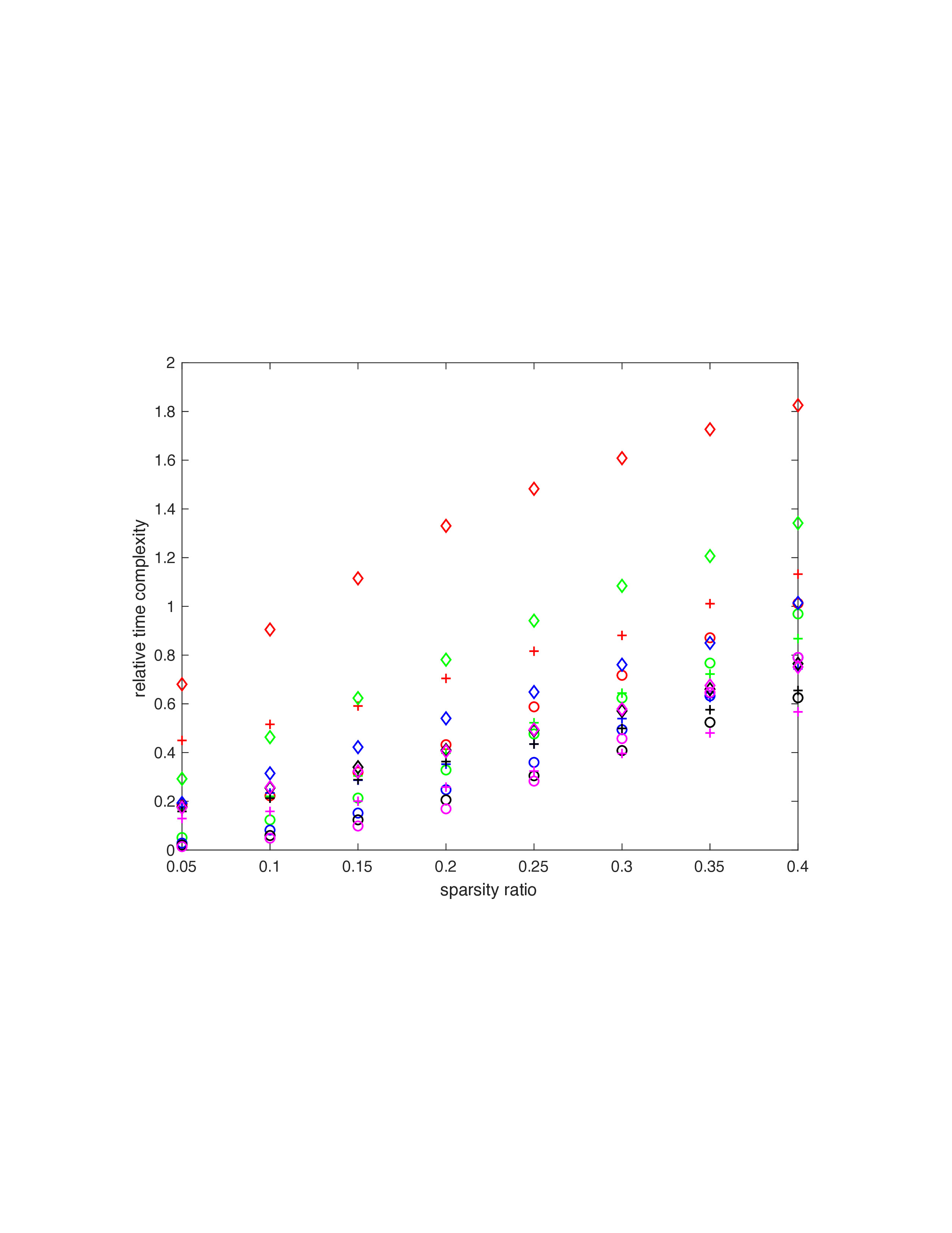
Table 1: Ratio of time complexity of FCSDTW over CDTW with varying sparsity ratios
\begin{minipage}[c]{1\linewidth}| data set | sparsity ratio | |||||
|---|---|---|---|---|---|---|
| 0.05 | 0.10 | 0.15 | 0.20 | 0.25 | 0.30 | |
| SC | 0.686 | 0.748 | 0.809 | 0.943 | 1.014 | 1.123 |
| DPT | 0.479 | 0.490 | 0.563 | 0.636 | 0.720 | 0.806 |
| ECG | 0.390 | 0.382 | 0.471 | 0.529 | 0.622 | 0.709 |
| 50W | 0.133 | 0.181 | 0.244 | 0.322 | 0.416 | 0.517 |
| TR | 0.140 | 0.180 | 0.241 | 0.320 | 0.420 | 0.520 |
| CF | 0.219 | 0.330 | 0.287 | 0.327 | 0.414 | 0.510 |
| BF | 0.209 | 0.227 | 0.281 | 0.358 | 0.442 | 0.526 |
| Car | 0.171 | 0.205 | 0.253 | 0.322 | 0.393 | 0.491 |
| L2 | 0.166 | 0.193 | 0.242 | 0.307 | 0.372 | 0.464 |
| WM | 0.151 | 0.167 | 0.206 | 0.255 | 0.320 | 0.387 |
| ML | 0.123 | 0.149 | 0.190 | 0.241 | 0.297 | 0.360 |
| CET | 0.127 | 0.156 | 0.193 | 0.245 | 0.303 | 0.371 |
| data set | length | \(b_{2}\) | \(b_{0}\) SC |
60 | 5.368 | 0.937 ECG |
96 | 4.290 | 0.496 50W |
270 | 4.478 | 0.199 TR |
275 | 4.332 | 0.205 CF |
286 | 3.586 | 0.289 BF |
470 | 3.745 | 0.168 Car |
577 | 3.463 | 0.205 L2 |
637 | 3.706 | 0.118 WM |
900 | 2.957 | 0.166 ML |
1024 | 3.036 | 0.205 CET |
1639 | 2.729 | 0.140 |
|---|
| data set | length | \(b_{2}\) | \(b_{0}\) \iffalse SC |
60 | 5.368 | 0.937 \fi ECG |
96 | 4.290 | 0.496 \iffalse 50W |
270 | 4.478 | 0.199 \fi TR |
275 | 4.332 | 0.205 \iffalse CF |
286 | 3.586 | 0.289 BF |
470 | 3.745 | 0.168 \fi Car |
577 | 3.463 | 0.205 \iffalse L2 |
637 | 3.706 | 0.118 WM |
900 | 2.957 | 0.166 \fi ML |
1024 | 3.036 | 0.205 CET |
1639 | 2.729 | 0.140 |
|---|
Table 2: Ratio of time complexity of FCSDTW over CSDTW with varying sparsity ratios
\begin{minipage}[c]{1\linewidth}| data set | sparsity ratio | |||||
|---|---|---|---|---|---|---|
| 0.05 | 0.10 | 0.15 | 0.20 | 0.25 | 0.30 | |
| SC | 0.562 | 0.491 | 0.466 | 0.443 | 0.449 | 0.460 |
| DPT | 0.421 | 0.476 | 0.466 | 0.459 | 0.468 | 0.473 |
| ECG | 0.357 | 0.386 | 0.378 | 0.420 | 0.429 | 0.432 |
| 50W | 0.478 | 0.393 | 0.394 | 0.412 | 0.437 | 0.479 |
| TR | 0.463 | 0.392 | 0.398 | 0.421 | 0.447 | 0.502 |
| CF | 0.259 | 0.235 | 0.224 | 0.252 | 0.461 | 0.483 |
| BF | 0.309 | 0.316 | 0.385 | 0.453 | 0.481 | 0.514 |
| Car | 0.929 | 0.674 | 0.620 | 0.602 | 0.622 | 0.651 |
| L2 | 0.933 | 0.669 | 0.522 | 0.628 | 0.644 | 0.673 |
| WM | 0.691 | 0.581 | 0.555 | 0.570 | 0.595 | 0.628 |
| ML | 0.690 | 0.588 | 0.569 | 0.584 | 0.612 | 0.603 |
| CET | 0.709 | 0.603 | 0.580 | 0.594 | 0.595 | 0.690 |
Table 3: Relative time complexity of CAWarp over CDTW with varying sparsity ratio
\begin{minipage}[c]{1\linewidth}| data set | sparsity ratio | |||||
|---|---|---|---|---|---|---|
| 0.05 | 0.10 | 0.15 | 0.20 | 0.25 | 0.30 | |
| SC | .237 | .330 | .413 | .555 | .683 | .862 |
| DPT | .170 | .231 | .338 | .454 | .576 | .719 |
| ECG | .144 | .197 | .289 | .404 | .554 | .647 |
| 50W | .0494 | .122 | .217 | .403 | .794 | .946 |
| TR | .0496 | .120 | .209 | .328 | .487 | .635 |
| CF | .0934 | .204 | .228 | .327 | .455 | .597 |
| BF | .052 | .0936 | .174 | .272 | .391 | .519 |
| Car | .0275 | .0773 | .150 | .245 | .349 | .484 |
| L2 | .0245 | .0686 | .138 | .229 | .321 | .454 |
| WM | .0167 | .052 | .103 | .175 | .258 | .359 |
| ML | .0153 | .0497 | .101 | .167 | .249 | .340 |
| CET | .0142 | .0488 | .102 | .173 | .260 | .359 |
Table 4: Relative error of CAWarp cost against constrained DTW cost with varying sparsity ratios in \(10^{-3}\)
\begin{minipage}[c]{1\linewidth}| data set | sparsity ratio | |||||
|---|---|---|---|---|---|---|
| 0.05 | 0.10 | 0.15 | 0.20 | 0.25 | 0.30 | |
| SC | 0 | 0 | 0 | 0 | 0 | 0 |
| DPT | 1.4 | 2.0 | 3.5 | 4.9 | 4.5 | 5.7 |
| ECG | 0.7 | 2.3 | 3.1 | 2.8 | 2.2 | 2.6 |
| 50W | 0.336 | 0.582 | 0.703 | 0.713 | 0.668 | 0.578 |
| TR | 0.133 | 0.409 | 0.634 | 0.838 | 0.590 | 0.325 |
| CF | 0 | 0 | 0.2 | 0.9 | 2.3 | 0 |
| BF | 0.406 | 0.609 | 0.344 | 0 | 0 | 0 |
| Car | 0.426 | 0.288 | 0.316 | 0.192 | 0.172 | 0.086 |
| L2 | 0.0457 | 0.0323 | 0 | 0 | 0 | 0 |
| WM | 0.048 | 0.106 | 0.171 | 0 | 0.023 | 0 |
| ML | 8.439 | 4.234 | 2.290 | 1.045 | 0.793 | 0.619 |
| CET | 0 | 0 | 0 | 0 | 0 | 0 |
Table 5: Relative errors of the cost of FCSDTW over CDTW with varying sparsity ratio in \(10^{-4}\) . The symbol `eps' stands for errors less than double precision accuracy in MATLAB.
\begin{minipage}[c]{1\linewidth}| data set | sparsity ratio | |||||||
|---|---|---|---|---|---|---|---|---|
| 0.05 | 0.10 | 0.15 | 0.20 | 0.25 | 0.30 | 0.35 | 0.40 | |
| \iffalse IPD | eps | eps | eps | eps | eps | 1.443 | ||
| \fi \iffalse SC | eps | eps | eps | 0.0260 | 4.049 | 1.742 | ||
| SRS | 0 | 0 | 0 | eps | 0 | eps | ||
| DPT | eps | 0.166 | eps | 1.327 | 1.978 | 2.999 | ||
| \fi ECG | eps | eps | eps | 0.0017 | 0.1039 | 0.0172 | 0.1733 | 1.2845 |
| \iffalse CBF | eps | eps | eps | eps | eps | 0.657 | ||
| EC5 | eps | 0 | eps | eps | eps | eps | ||
| 50W | eps | 0.0189 | 0.135 | 0.320 | 0.323 | 0.577 | ||
| \fi TR | eps | eps | eps | 0.0769 | 0.0940 | 0.0789 | 0.0345 | 0.0474 |
| \iffalse CF | eps | eps | eps | 6.874 | 0.0148 | 0.0476 | ||
| BF | eps | 0 | 0 | 0 | 0.0494 | 0.326 | ||
| OO | eps | eps | eps | 1.328 | 1.072 | 3.264 | ||
| \fi Car | eps | eps | 0.0673 | 0.0586 | 0.2367 | 0.2328 | 0.7437 | 0.3674 |
| \iffalse L2 | eps | eps | 0.0576 | 0.181 | 0.332 | 1.045 | ||
| WM | eps | eps | eps | 0.468 | 0.662 | 0.455 | ||
| \fi ML | eps | 0.0250 | 0.0464 | 0.0364 | 0.1336 | 0.5085 | 0.1859 | 0.3958 |
| CET | eps | eps | 0.0023 | 0.0293 | 0.0384 | 0.0710 | 0.1065 | 0.2563 |
Table 6: Relative errors of the cost of CAWarp over CDTW cost with varying sparsity ratio.
\begin{minipage}[c]{1\linewidth}| data set | sparsity ratio | |||||||
|---|---|---|---|---|---|---|---|---|
| 0.05 | 0.10 | 0.15 | 0.20 | 0.25 | 0.30 | 0.35 | 0.40 | |
| \iffalse IPD | 33.094 | 24.959 | 89.640 | 165.520 | 139.971 | 82.659 | ||
| SC | 150.857 | 625.671 | 540.534 | 645.174 | 794.070 | 844.856 | ||
| SRS | 0 | 0 | 241.207 | 46.267 | 157.735 | 43.886 | ||
| DPT | 177.505 | 111.074 | 228.100 | 197.067 | 193.190 | 170.947 | ||
| \fi ECG | 0.3053 | 0.2553 | 0.2363 | 0.1898 | 0.1681 | 0.1608 | 0.1634 | 0.1494 |
| \iffalse CBF | 383.840 | 420.609 | 283.245 | 587.533 | 406.610 | 411.291 | ||
| EC5 | eps | eps | 468.466 | 74.623 | 1.357 | 387.677 | ||
| 50W | 5.589 | 13.984 | 19.434 | 21.219 | 26.105 | 30.290 | ||
| \fi TR | 0.3998 | 0.3534 | 0.3273 | 0.2938 | 0.2878 | 0.2673 | 0.2470 | 0.2467 |
| \iffalse CF | 4.476 | 10.489 | 25.657 | 67.956 | 39.095 | 38.563 | ||
| BF | 0.352 | 23.153 | 9.272 | 11.770 | 3.634 | 32.058 | ||
| OO | 3.288 | 33.644 | 131.998 | 163.406 | 196.390 | 258.514 | ||
| \fi Car | 0.2476 | 0.1664 | 0.1671 | 0.1342 | 0.1476 | 0.1407 | 0.1497 | 0.1312 |
| \iffalse L2 | 25.328 | 92.240 | 106.789 | 146.288 | 176.498 | 204.591 | ||
| WM | 0.129 | 1.059 | 3.810 | 7.422 | 15.104 | 24.074 | ||
| \fi ML | 0.2004 | 0.1402 | 0.1092 | 0.1018 | 0.0910 | 0.0810 | 0.0689 | 0.0714 |
| CET | 0.3627 | 0.3101 | 0.2927 | 0.2851 | 0.2089 | 0.2300 | 0.2126 | 0.2065 |
Table 7: Relative time complexity of CAWarp over constrained DTW with varying sparsity ratio
\begin{minipage}[c]{1\linewidth}| data set | sparsity ratio | |||||
|---|---|---|---|---|---|---|
| 0.05 | 0.10 | 0.15 | 0.20 | 0.25 | 0.30 | |
| IPD | 0.126 | 0.252 | 0.362 | 0.477 | 0.564 | 0.655 |
| SC | 0.0756 | 0.135 | 0.211 | 0.318 | 0.414 | 0.602 |
| SRS | 0.126 | 0.106 | 0.198 | 0.359 | 0.486 | 0.633 |
| DPT | .0564 | 0.111 | 0.197 | 0.297 | 0.401 | 0.534 |
| ECG | .0494 | 0.102 | 0.186 | 0.277 | 0.406 | 0.498 |
| CBF | 0.0485 | 0.0945 | 0.157 | 0.259 | 0.371 | 0.485 |
| EC5 | 0.0645 | 0.0912 | 0.168 | 0.250 | 0.375 | 0.475 |
| 50W | 0.0229 | 0.0737 | 0.144 | 0.231 | 0.338 | 0.449 |
| TR | 0.0251 | 0.0732 | 0.144 | 0.231 | 0.345 | 0.466 |
| CF | 0.0269 | 0.0736 | 0.144 | 0.222 | 0.340 | 0.449 |
| BF | 0.0215 | 0.0634 | 0.134 | 0.217 | 0.318 | 0.427 |
| OO | 0.0193 | 0.0600 | 0.141 | 0.218 | 0.318 | 0.424 |
| Car | 0.0199 | 0.0651 | 0.134 | 0.223 | 0.320 | 0.451 |
| L2 | 0.0189 | 0.0604 | 0.129 | 0.213 | 0.303 | 0.423 |
| WM | 0.0172 | 0.0611 | 0.124 | 0.219 | 0.303 | 0.417 |
| ML | 0.0177 | 0.0633 | 0.132 | 0.217 | 0.324 | 0.427 |
| CET | 0.0179 | 0.066 | 0.137 | 0.231 | 0.324 | 0.445 |
Table 8: Comparison of ratios of time complexity among constrained SDTW, PrunedDTW and AWarp against constrained DTW for NHANES data
| sparsity ratio | 0.08333 | 0.125 | 0.16667 | 0.20833 | 0.250 | 0.29167 | 0.33333 SDTW |
1.3259 | 1.6004 | 1.8779 | 2.0180 | 2.1822 | 2.2949 | 2.4506 PrunedDTW |
1.3720 | 1.4382 | 1.4313 | 1.4336 | 1.4365 | 1.4446 | 1.4643 |
|---|---|---|---|---|---|---|---|---|---|---|---|---|---|---|---|---|---|---|---|---|---|
| AWarp | 0.2232 | 0.3139 | 0.4079 | 0.4925 | 0.5861 | 0.6669 | 0.7825 | ||||||||||||||
| error of the cost(AWarp) | 18.2608 | 7.0270 | 5.8522 | 5.6250 | 6.1608 | 7.0407 | 9.2129 |
Table 9: Comparison of the relative time complexities of CAWarp, CSDTW, and FCSDTW against CDTW
| class | 3 | 7 |
|---|---|---|
| sparsity ratio | 0.0578 | 0.02697 |
| CSDTW | 0.2204 | 0.1672 |
| FCSDTW | 0.1426 | 0.1362 |
| CAWarp | 0.0350 | 0.0194 |
Table 10: Regression results of relative time complexity of constrained SDTW against sparsity ratio up to 0.1
| train data set | length | \(b_{1}\) | \(b_{0}\) synthetic control |
61 | 4.8913 | 0.2745 CBF |
129 | 5.6920 | 0.0727 50 words |
271 | 5.9246 | 0.0040 Beef |
471 | 5.4744 | 0.0069 MALLAT |
1025 | 5.2093 | -0.0056 |
|---|
6. Conclusion
This study developed and analyzed FCSDTW to compare sparse time series with zero data in many research applications. FCSDTW closely approximated CDTW with much lower time complexities for time series with many zero values and especially large lengths. \iffalse This study shows computational complexity of FCSDTW can be significantly reduced with a small sparsity ratio and large lengths. \fi FCSDTW is a distinct algorithm from other approaches producing huge complexity reduction with significant errors or no change in complexity without error. Further numerical experiments support the efficiency of FCSDTW compared against CSDTW and CAWarp. \iffalse FCSDTW has been developed and analyzed to utilize sparse time series when managing zero data in many research applications. FCSDTW closely approximate CDTW with much less computational burden for sparse time series. This study shows its computational complexity can be significantly reduced with a small sparsity ratio and large lengths. FCSDTW is a distinct algorithm from other approaches producing huge complexity reduction with significant errors or no change in complexity without error. Further numerical experiments support the efficiency of FCSDTW compared against CSDTW and CAWarp. \fi \iffalse FCSDTW has been developed and analyzed to utilize sparse time series when managing zero data in many research applications. FCSDTW is closely approximate to CDTW and can find the same solution with less computation for sparse time series. Its computational complexity is proportional to the square of the sparsity ratio and can yield significant decreases for time series with small enough sparsity ratio and large enough lengths. FCSDTW is different than other approaches which modify the time series and/or the DTW algorithm in a way which does not focus on the sparse structure. These methods can yield large complexity reduction but at the expense of increased error or can yield no complexity reduction without any error. Numerical experiments from synthetic and real data support the analysis that FCSDTW is faster than CSDTW for the sparse time series. This work provides a framework to combine FCSDTW with these other complexity reduction approaches. \fiReferences
[1]. Hiroaki Sakoe and Seibi Chiba. Dynamic programming algorithm optimization for spoken word recognition. IEEE Transactions on Acoustics, Speech and Signal Processing, 26(1):43–49, 1978.
[2]. Claus Bahlmann and Hans Burkhardt. The writer independent online handwriting recognition system frog on hand and cluster generative statistical dynamic time warping. IEEE Transactions on Pattern Analysis and Machine Intelligence, 26(3):299–310, 2004.
[3]. Zsolt Miklos Kovacs-Vajna. A fingerprint verification system based on triangular matching and dynamic time warping. IEEE Transactions on Pattern Analysis and Machine Intelligence, 22(11):1266–1276, 2000.
[4]. Samsu Sempena, Nur Ulfa Maulidevi, and Peb Ruswono Aryan. Human action recognition using dynamic time warping. In Proceedings of the 2011 International Conference on Electrical Engineering and Informatics, pages 1–5. IEEE, 2011.
[5]. Philippe Esling and Carlos Agon. Time-series data mining. ACM Computing Surveys (CSUR), 45(1):12, 2012.
[6]. Tak-chung Fu. A review on time series data mining. Engineering Applications of Artificial Intelligence, 24(1):164–181, 2011.
[7]. Youngha Hwang and Saul B Gelfand. Constrained sparse dynamic time warping. In International Conference on Machine Learning and Applications, pages 216–222. IEEE, 2018.
[8]. Youngha Hwang and Saul B Gelfand. Fast sparse dynamic time warping. In 2022 26th International Conference on Pattern Recognition (ICPR), pages 3872–3877. IEEE, 2022.
[9]. Heather A Eicher-Miller, Saul Gelfand, Youngha Hwang, Edward Delp, Anindya Bhadra, and Jiaqi Guo. Distance metrics optimized for clustering temporal dietary patterning among us adults. Appetite, 144:104451, 2020.
[10]. David Murray and L Stankovic. Refit: electrical load measurements. URL= http://www.refitsmarthomes.org/, 2017.
[11]. Youngha Hwang and Saul B Gelfand. Sparse dynamic time warping. In International Conference on Machine Learning and Data Mining in Pattern Recognition, pages 163–175. Springer, 2017.
[12]. Youngha Hwang and Saul B Gelfand. Binary sparse dynamic time warping. In International Conference on Machine Learning and Data Mining in Pattern Recognition, pages 748–759. Springer, 2019.
[13]. Youngha Hwang. Constrained binary sparse dynamic time warping. In manuscript.
[14]. Abdullah Mueen, Nikan Chavoshi, Noor Abu-El-Rub, Hossein Hamooni, Amanda Minnich, and Jonathan MacCarthy. Speeding up dynamic time warping distance for sparse time series data. Knowledge and Information Systems, 54(1):237–263, 2018.
[15]. Eamonn Keogh, Xiaopeng Xi, Li Wei, and Chotirat Ann Ratanamahatana. The ucr time series classification/clustering homepage. URL= http://www.cs.ucr.edu/˜ eamonn/time series data, 2006.
Cite this article
Hwang,Y. (2024). Fast Constrained Sparse Dynamic Time Warping. Applied and Computational Engineering,120,50-58.
Data availability
The datasets used and/or analyzed during the current study will be available from the authors upon reasonable request.
Disclaimer/Publisher's Note
The statements, opinions and data contained in all publications are solely those of the individual author(s) and contributor(s) and not of EWA Publishing and/or the editor(s). EWA Publishing and/or the editor(s) disclaim responsibility for any injury to people or property resulting from any ideas, methods, instructions or products referred to in the content.
About volume
Volume title: Proceedings of the 5th International Conference on Signal Processing and Machine Learning
© 2024 by the author(s). Licensee EWA Publishing, Oxford, UK. This article is an open access article distributed under the terms and
conditions of the Creative Commons Attribution (CC BY) license. Authors who
publish this series agree to the following terms:
1. Authors retain copyright and grant the series right of first publication with the work simultaneously licensed under a Creative Commons
Attribution License that allows others to share the work with an acknowledgment of the work's authorship and initial publication in this
series.
2. Authors are able to enter into separate, additional contractual arrangements for the non-exclusive distribution of the series's published
version of the work (e.g., post it to an institutional repository or publish it in a book), with an acknowledgment of its initial
publication in this series.
3. Authors are permitted and encouraged to post their work online (e.g., in institutional repositories or on their website) prior to and
during the submission process, as it can lead to productive exchanges, as well as earlier and greater citation of published work (See
Open access policy for details).
References
[1]. Hiroaki Sakoe and Seibi Chiba. Dynamic programming algorithm optimization for spoken word recognition. IEEE Transactions on Acoustics, Speech and Signal Processing, 26(1):43–49, 1978.
[2]. Claus Bahlmann and Hans Burkhardt. The writer independent online handwriting recognition system frog on hand and cluster generative statistical dynamic time warping. IEEE Transactions on Pattern Analysis and Machine Intelligence, 26(3):299–310, 2004.
[3]. Zsolt Miklos Kovacs-Vajna. A fingerprint verification system based on triangular matching and dynamic time warping. IEEE Transactions on Pattern Analysis and Machine Intelligence, 22(11):1266–1276, 2000.
[4]. Samsu Sempena, Nur Ulfa Maulidevi, and Peb Ruswono Aryan. Human action recognition using dynamic time warping. In Proceedings of the 2011 International Conference on Electrical Engineering and Informatics, pages 1–5. IEEE, 2011.
[5]. Philippe Esling and Carlos Agon. Time-series data mining. ACM Computing Surveys (CSUR), 45(1):12, 2012.
[6]. Tak-chung Fu. A review on time series data mining. Engineering Applications of Artificial Intelligence, 24(1):164–181, 2011.
[7]. Youngha Hwang and Saul B Gelfand. Constrained sparse dynamic time warping. In International Conference on Machine Learning and Applications, pages 216–222. IEEE, 2018.
[8]. Youngha Hwang and Saul B Gelfand. Fast sparse dynamic time warping. In 2022 26th International Conference on Pattern Recognition (ICPR), pages 3872–3877. IEEE, 2022.
[9]. Heather A Eicher-Miller, Saul Gelfand, Youngha Hwang, Edward Delp, Anindya Bhadra, and Jiaqi Guo. Distance metrics optimized for clustering temporal dietary patterning among us adults. Appetite, 144:104451, 2020.
[10]. David Murray and L Stankovic. Refit: electrical load measurements. URL= http://www.refitsmarthomes.org/, 2017.
[11]. Youngha Hwang and Saul B Gelfand. Sparse dynamic time warping. In International Conference on Machine Learning and Data Mining in Pattern Recognition, pages 163–175. Springer, 2017.
[12]. Youngha Hwang and Saul B Gelfand. Binary sparse dynamic time warping. In International Conference on Machine Learning and Data Mining in Pattern Recognition, pages 748–759. Springer, 2019.
[13]. Youngha Hwang. Constrained binary sparse dynamic time warping. In manuscript.
[14]. Abdullah Mueen, Nikan Chavoshi, Noor Abu-El-Rub, Hossein Hamooni, Amanda Minnich, and Jonathan MacCarthy. Speeding up dynamic time warping distance for sparse time series data. Knowledge and Information Systems, 54(1):237–263, 2018.
[15]. Eamonn Keogh, Xiaopeng Xi, Li Wei, and Chotirat Ann Ratanamahatana. The ucr time series classification/clustering homepage. URL= http://www.cs.ucr.edu/˜ eamonn/time series data, 2006.