1. Introduction

Discrepancies between the current automatic feature analysis of CTG signals and expert consensus arise from differences in fetal heart rate baseline and expert interpretation. The error in baseline interpretation of fetal heart rate can also affect the interpretation of acceleration and deceleration zones, and the differences in their judgments were interdependent. According to the clinical definitions of fetal heart rate baseline, acceleration, and deceleration, the deceleration and acceleration parts in the FHR signal were removed, and the remaining modules were used for baseline calculation; After determining the baseline, the acceleration and deceleration zones were calculated based on the difference between the baseline and the signal, forming a logical dead loop.

Currently, the mainstream method for signal feature analysis of CTG is still based on signal processing methods, which use sliding window filtering and progressive waveform trimming strategies to locate the acceleration and deceleration regions, from which the signal baseline is then derived [1]. Despite their widespread use, these methods face limitations and fail to achieve consistent, accurate results.

The existing methods cannot achieve satisfactory results. Popular deep learning methods and relevant network models were introduced to handle the automatic feature extraction problem of FHR signals. Deep learning has shown good performance in morphological feature extraction, offers promising alternatives for tackling these challenges. For the localization of acceleration and deceleration zones, deep learning was used to process time-series signals for segmentation and identification of acceleration and deceleration zones. For the baseline calculation module, a baseline calculation strategy based on long short-term filters was proposed. This approach integrates morphological features with temporal priors, aligning closely with the clinical methodology used by doctors to determine baselines.

In summary, this study algorithm for CTG signal feature extraction uses deep learning, addressing existing limitations and enhancing accuracy in signal analysis.

2. Test dataset

The French Lille database and Overseas Chinese Hospital database were used to verify the performance of the feature automatic extraction algorithm for FHR signals in CTG signals based on EADU-Net proposed.

3. Feature extraction algorithm for EADU-Net

An integrated U-shaped network equipped with a CBAM attention mechanism and Dense-block module for automatic feature extraction of FHR signals was proposed. The process can be roughly divided into 3 steps:

(1) The preprocessing and enhancement of data remove noise from the signal, and the dataset was enhanced and expanded through cropping and concatenation.

(2) EDAU-Net was used to segment the signal segments into areas of fetal heart rate acceleration and deceleration, and then concatenating the pre-labeled sub-segments to obtain a complete estimated signal annotated by the network.

(3) The method of filtering with long and short line filters was used to obtain the baseline fetal heart rate of the signal, and finally provide the marked fetal heart rate acceleration and acceleration zone, as well as the baseline fetal heart rate of the entire segment [2].

3.1. EADU-Net Architecture

Deep learning was used to automatically segment acceleration/deceleration regions during acceleration/deceleration detection. The input of the neural network was the preprocessed FHR signal sub-segment. EADU-Net consists of four U-Nets (ADU-Nets) with attention mechanism and Dense-block, with kernel sizes (KS) of 21, 31, 61, and 81, respectively. By integrating the predicted results of the four MAU-Nets using the "OR" operation, potential acceleration/deceleration point areas in the signal sub-segments can be detected, as shown in the following figure.

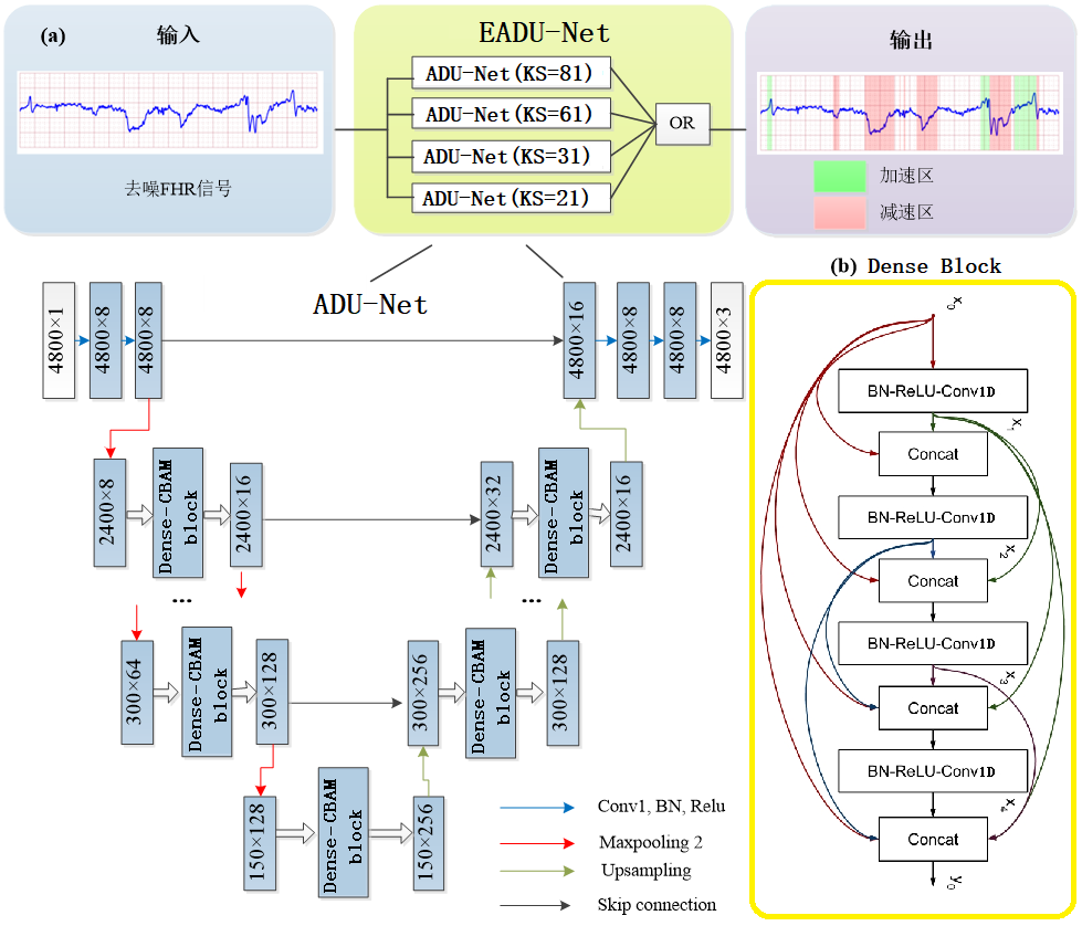
Figure 1: Structure of EADU-Net

The ADU-NET network structure is shown in the above figure, with the main body composed of U-net, which can be clearly divided into the encoder module on the left and the decoder module on the right, with the encoder and decoder modules connected in the middle.

The input data is one-dimensional signal data, with a length of 4,800 and 1 channel. The selected data batch size is 64.

Finally, after passing through a layer of softmax function, the output data length is 4,800 and the channels are 3, representing the segmentation of the baseline, acceleration, and deceleration regions in the CTG.

3.2. Loss Function and Optimizer

A comprehensive loss function was used, including Cross-Entropy (CE), Generalized- Dice (GD), and Kullback-Leibler (KL), and these three parts are combined with certain weights. The respective weights are shown in the following formula.

\( LOSS=0.99GD+0.01CE+0.01KL \) (1)

The classic Adam optimizer was used to set the initial learning rate of the model at 0.001 during training. After every 50 iteration cycles, the learning rate decays by 0.1 times, for a total of 210 training epochs.

3.3. Automatic baseline calculation

After predicting and identifying the acceleration and deceleration zones through the sub-segments of the network, the individual customizations were concatenated in the above manner to obtain the overall signal acceleration and deceleration zone prediction results. The complete signal obtained by concatenating the predicted indicators is the basis for automatic baseline calculation in this article [3].

Firstly, based on the previous prediction, the preprocessed FHR signal x [n] and its predicted label y [n] were obtained (Figure 3-5b), n=1, 2, ..., N. Then, the discrete baseline state signal L [n] was calculated as follows:

\( L[n]=\begin{cases} \begin{array}{c} x[n], y[n]=1 \\ 0, y[n]=0 \end{array} \end{cases} \) (2)

Next, long-term median filtering was used to calculate the reference baseline L_ref [n], as follows:

\( {L_{ref}}[n]=\begin{cases} \begin{array}{c} median(L[n],⋯,L[n+k]), s[n]≥0.1 \\ 0, others \end{array} \end{cases} \) (3)

\( s[n]=\frac{1}{k}\sum _{i=n}^{n+k}y[i] \) (4)

Where, k is the window function length of the filter, set to 20 min. In this study, and s [n] is the percentage of baseline points in the sliding window. If there are few baseline points, the FHR reference baseline may be inaccurately calculated. Therefore, points with s [n] ≤ 0.1 are defined as invalid points and replaced with linear interpolation [4]. Next, compared with L_ref, baseline points in L [n] with fluctuations exceeding 15 bpm are identified as abnormal and removed. The calculation method is as follows:

\( L \prime [n]=\begin{cases} \begin{array}{c} L[n], |L[n]-{L_{ref}}[n]|≤15bpm \\ 0, others \end{array} \end{cases} \) (5)

Then, the outliers with values of 0 in L’ [n] are processed through linear interpolation. Finally, L’ [n] passes through a short-term median filter with a window function length of 2 min. to obtain the final baseline.

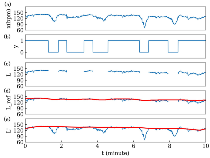
Figure 2: Schematic figure of automatic baseline calculation

3.4. Evaluation indicators

To evaluate the inconsistency between feature extraction methods and expert consensus, the test results were compared with expert consensus using the following metrics for each independent signal, as shown below.

Table 1: Explanation of Evaluation Index Parameters

To evaluate the differences between the algorithm feature extraction and expert annotation, the following five indicators were proposed. Three indicators reflect the performance of three different feature predictions, while the other two are comprehensive indicators, each of which simultaneously characterizes the performance of extracting and analyzing multiple features.

3.4.1. Baseline assessment

Baseline root mean square deviation (BL. RMSD) was approximately defined as the probability-based root mean square deviation, a measure of average deviation measured in bpm. Because the meaning was close to the variance, the smaller the fixed value, the better the representation performance. The specific formula is as follows [5]:

\( BL.RMSD(BL.P-BL.E)=\sqrt[]{\frac{\sum _{i=1}^{n}{({BL.P_{i}}-{BL.E_{i}})^{2}}}{n}} \) (6)

BL. P is the prediction baseline of the model, BL. E is the consensus marker baseline of experts, and n represents the number of FHR signal points in the segment.

3.4.2. Acceleration and deceleration detection

Acceleration and deceleration have similarities in morphology, and the F-measure is used to evaluate the accuracy of the algorithm's predicted acceleration and deceleration zones. The criterion for judgment is that the acceleration and deceleration zones segmented by the model are consistent with the expert's annotation results for more than 5s, which is considered positive. The specific formula is shown below.

\( F-Measure=\frac{2×PPV×SEN}{PPV+SEN} \) (7)

Where, the sensitivity of acceleration/deceleration detection (Acc.SEN/Dec.SEN) corresponds to the percentage of correctly detected acceleration/deceleration to the total number of acceleration/ deceleration recognized by expert consensus. The positive prediction of acceleration/deceleration detection (Acc. PPV/Dec. PPV) corresponds to the percentage of correctly detected acceleration/deceleration to the total number of acceleration/ deceleration detected by the algorithm [6].

3.4.3. Comprehensive evaluation indicators

The evaluation index SI integrates the accuracy of acceleration and deceleration event prediction and is the weighted sum and re-normalization of the acceleration and deceleration prediction performance results. The indicator considers the prediction quality of acceleration and deceleration from quantity, location, and area, and the percentage difference between the predicted results and expert identification for acceleration and deceleration was calculated. Therefore, the smaller the indicator value, the better the performance. The specific formula is shown below.

\( SI=\frac{ASI+2DSI}{3} \) (8)

\( ASI=\sqrt[]{\frac{\sum _{i=1}^{A}{({Acc.P_{i}}-{Acc.E_{i}})^{2}}}{\sum _{i=1}^{A}{max({Acc.P_{i}},{Acc.E_{i}})^{2}}}}×100\% \) (9)

\( DSI=\sqrt[]{\frac{\sum _{i=1}^{D}{({Dec.P_{i}}-{Dec.E_{i}})^{2}}}{\sum _{i=1}^{D}{max({Dec.P_{i}},{Dec.E_{i}})^{2}}}}×100\% \) (10)

MADI appears to be a rough assessment of the morphological differences between both baselines for prediction and sample identification over time series. The smaller the indicator value, the better the performance. The specific formula is shown below.

\( MADI=\frac{1}{n}\sum _{i=1}^{n}\frac{{({BL.P_{i}}-{BL.E_{i}})^{2}}}{{(D_{FHR}^{BL.P})_{i}} × {(D_{FHR}^{BL.E})_{i}} + {({BL.P_{i}}-{BL.E_{i}})^{2}}} \) (11)

\( {(D_{FHR}^{x})_{i}}= α+\sqrt[]{\frac{\sum _{j=i-120}^{i+120}{({x_{j}}-{FHR_{j}})^{2}}}{240}} \) (12)

Where, BL. P and BL.E are the predicted baseline and expert annotated baseline of the algorithm, respectively, and n is the total data volume of the FHR signal (the signal is 240 data volumes per minute, i.e. 4Hz). \( The average fetal heart rate variability of D_{FHR}^{x} \) within 1 min. around the current sample (using baseline x as a reference).

3.5. Results

The model for this test was built on Python using a Keras backend based on the TensorFlow framework.

Among the above indicators, higher values for Dec. F-measure and Acc. F-measure indicate better method performance, whereas lower values for BL. RMSD, SI, and MADI signify superior outcomes. By comparing the judgment results generated by different automatic analysis methods with those generated by expert consensus, the study reveals the inconsistencies between algorithm predictions and expert consensus. The median values [95% confidence intervals] of the five indicators mentioned above were calculated for comparison.

The 331 test datasets from the Huayi database were used to validate the accuracy and generalization of the model. Furthermore, to gain a clearer and more intuitive understanding of the performance of the model proposed based on deep learning methods, the WMFB algorithm, which currently has the best comprehensive performance, was used to compare five performance indicators. Additionally, the performance of the model parameters obtained using only U-net was also tested to visually demonstrate the basic performance of deep learning algorithms.

Table 2: Comparison between EADU-Net and WMFB methods

The test data shows in table 2 that the EADU-NET model proposed achieves higher performance in five indicators (including two comprehensive evaluation indicators and three single evaluation indicators). At the same time, the performance of the basic deep learning model U-net is not inferior to the currently known optimal WMFB algorithm.

4. Conclusion

A detailed description of the process of using deep learning's EDAU-Net was provided for automatic feature extraction of FHR signals. The training and validation phases utilized 66 expert annotated data from the French Lille Database, while 331 data from Overseas Chinese Hospital were used to test the network's feature analysis performance. Specific filtering was used to address the noise introduced in clinical signal acquisition. The filtered data was cropped to obtain enhanced data sub-segments from the signal data due to the issue of varying recording times and excessively long recording times. Theses sub-segments were then fed into the neural network for predicting and locating the acceleration and deceleration regions. The predicted data from the network was obtained, and the processed data was concatenated in a certain way, Subsequently, an automatic baseline calculation was performed. The baseline calculation principle was based on the quadratic filtering of both filters, long-term and short-term, to obtain the predicted fetal heart rate baseline under the network algorithm.

The performance of FHR signal feature extraction was evaluated based on EDAU-Net using five indicators to assess the performance of feature analysis. The five performance indicators of the network proposed were superior to the WMFB algorithm compared with the WMFB algorithm, which has the best performance among traditional methods. The results indicated that the network proposed has higher performance, with feature analysis results obtained by the algorithm showing the smallest difference from the expert's interpretation results.

References

[1]. Huang M.J. Study and Implementation of Fetal Electronic Monitoring Analysis Algorithm Technology [D] Jinan University, 2021.DOI: 10.27167/d.cnki.gjinu.2019.000144
[2]. Yin X.H., Wang Y.C., Li D.Y. A review of medical image segmentation techniques based on U-Net structure improvement [J] Journal of Software, 2021,32
[3]. BOUDET S, DE L’AULNOIT A H, DEMAILLY R, et al. Fetal heart rate baseline computation with a weighted median filter [J]. Computers in Biology and Medicine, 2019, 114: 103468.
[4]. Huang X.C. Study on Feature Parameter Extraction and Fetal Condition Evaluation Method Based on CTG [D] Jinan University, 2021.DOI: 10.27167/d.cnki.gjinu.2019.000166
[5]. Liu W.Y., Wen Y.D., Yu Z.D. and Yang M. “Large-Margin Softmax Loss for Convolutional Neural Networks.” International Conference on Machine Learning (2016).
[6]. S. Guan, A. A. Khan, S. Sikdar and P. V. Chitnis, "Fully Dense UNet for 2-D Sparse Photoacoustic Tomography Artifact Removal," in IEEE Journal of Biomedical and Health Informatics, vol. 24, no. 2, pp. 568-576, Feb. 2020, doi: 10.1109/JBHI.2019.2912935.
Cite this article
Chen,L. (2024). Research on CTG Feature Extraction Algorithm Based on Deep Learning. Applied and Computational Engineering,120,120-126.
Data availability
The datasets used and/or analyzed during the current study will be available from the authors upon reasonable request.
Disclaimer/Publisher's Note
The statements, opinions and data contained in all publications are solely those of the individual author(s) and contributor(s) and not of EWA Publishing and/or the editor(s). EWA Publishing and/or the editor(s) disclaim responsibility for any injury to people or property resulting from any ideas, methods, instructions or products referred to in the content.
About volume
Volume title: Proceedings of the 5th International Conference on Signal Processing and Machine Learning
© 2024 by the author(s). Licensee EWA Publishing, Oxford, UK. This article is an open access article distributed under the terms and
conditions of the Creative Commons Attribution (CC BY) license. Authors who
publish this series agree to the following terms:
1. Authors retain copyright and grant the series right of first publication with the work simultaneously licensed under a Creative Commons
Attribution License that allows others to share the work with an acknowledgment of the work's authorship and initial publication in this
series.
2. Authors are able to enter into separate, additional contractual arrangements for the non-exclusive distribution of the series's published
version of the work (e.g., post it to an institutional repository or publish it in a book), with an acknowledgment of its initial
publication in this series.
3. Authors are permitted and encouraged to post their work online (e.g., in institutional repositories or on their website) prior to and
during the submission process, as it can lead to productive exchanges, as well as earlier and greater citation of published work (See
Open access policy for details).