1. Introduction

In the financial sector, analyzing bank term deposit data is significant, especially in optimizing marketing strategies and enhancing customer loyalty. By examining customers' financial status, age, profession, and income level, banks can identify customer segments more likely to subscribe to term deposits, allowing for more targeted marketing efforts [1]. Additionally, term deposits provide a stable source of funds, and by analyzing deposit data, banks can better forecast funding needs and allocate resources to balance liquidity and profitability [2].

With the advancement of artificial intelligence technology, complex ML models, like deep neural networks and random forests, have recently achieved significant results in bank marketing [3-6]. However, due to their complex internal structures and nonlinear characteristics, these so-called "black box" models’ decision-making procedures are mostly challenging to comprehend. More trust in the model’s ouput is required as a result of this opacity, especially in high-risk fields such as healthcare, finance, and autonomous driving. Therefore, conducting in-depth research on the interpretability of ML models is essential. This not only helps to understand the basis of model decisions, but also improves the model’s credibility and transparency, avoiding bias and discrimination and thereby better serving practical applications.

To ensure the fairness and reliability of the final decisions, this paper employs multiple ML models to predict outcomes on a bank term deposit dataset, selecting the best-performing model for further in-depth analysis. In addition, the model's interpretability is assessed by the SHAP [7] analysis, revealing features that influence the prediction results and their contributions to the model's decisions. This approach offers a more transparent and comprehensible analysis, meeting increasingly strict regulatory requirements and helping the bank better understand the model's decision-making logic, ultimately optimizing strategies [8].

After the introduction, this paper unfolds through a structured sequence of sections. We initiate a brief literature review of previous works, then focus on the methodology employed for predicting bank term deposits, highlighting the selection and implementation of various ML models. Following this, the results of the SHAP analysis will be presented to demonstrate the key factors influencing model predictions. Finally, a short conclusion will be made.

2. Literature Review

2.1. Customer behavior insights to enhance banking decisions

Understanding customer behavior is crucial in the banking industry, as accurate insights into customer characteristics and needs can help improve marketing strategies, enhance customer retention, and manage financial risks. One critical approach is clustering analysis, which groups customers based on shared characteristics to optimize resource allocation and enable tailored financial products. Using time series clustering, Abbasimehr and Shabani [1] proposed a dynamic approach for customer segmentation. They identified key customer groups such as 'high-value growing' and 'churn-prone' segments, allowing tailored strategies for each group. Calvo-Porral and Lévy-Mangin [9] categorized bank customers based on emotions experienced during service interactions into groups including 'angry complainers' and 'happy satisfied.' This method proved significant for predicting behaviors like loyalty and complaint likelihood.

Another crucial area is credit scoring, where banks evaluate customer creditworthiness to reduce default risk. Recent studies have introduced hybrid models to improve accuracy without sacrificing clarity. A deep genetic hierarchical network was developed by Pławiak et al. [10], demonstrating the state-of-the-art accuracy. Dumitrescu et al. [11] created the penalized logistic tree regression model, integrating decision-tree features into logistic regression to capture complex patterns that standard logistic regression might overlook. Nevertheless, de Lima Lemos et al. [12] predicted customer churn using a comprehensive dataset from a large Brazilian bank.

2.2. Predicting deposit subscription based on ML

ML has emerged as a critical approach in predicting customer deposit subscriptions, offering banks advanced tools to analyze complex datasets and improve decision-making through more accurate and data-driven predictions. Lu et al. [5] developed an artificial immune network (AIN), which was enhanced by feature selection, demonstrating improved accuracy and effectiveness in addressing class imbalance issues within financial recommendation systems. By refining the S_Kohonen network, Yan et al. [6] presented an enhanced whale optimization algorithm, demonstrating significant improvements in classification accuracy of successful bank telephone marketing. Ghatasheh et al. [4] enhanced the accuracy of predicting bank clients' response to term deposit products in imbalanced datasets by employing cost-sensitive analysis and artificial neural networks, offering data-driven insights for telemarketing decisions in the banking industry. Feng et al. [3] introduced dynamic ensemble selection, which integrates precision and profit maximization for predicting bank telemarketing sales success.

While ML models have demonstrated superior accuracy in predicting customer deposit subscriptions, Carvalho et al. [13] emphasized that the internal logic and workings of these ‘black boxes’ remain difficult for users and experts to understand. This challenge highlights the growing need for interpretability techniques that can explain complex models without compromising their predictive power, leading to increased focus on interpretability analysis in ML applications.

2.3. Interpretability analysis for ML

The ability to provide meaning in a way that people can comprehend is known as interpretability [14]. Various interpretability methods have emerged in recent years to clarify how ML methods make decisions. LIME (Local Interpretable Model-agnostic Explanations) [15] approximates complex models locally with simpler, interpretable models to evaluate how individual features affect particular prediction. Its flexibility makes it suitable for a wide range of models, but it primarily offers local explanations, which limits its ability to provide consistent global insights.

SHAP [7] builds on Shapley values from game theory, providing a unified framework to attribute each feature’s contribution to the model result. Unlike LIME, it ensures consistency by delivering local and global explanations, allowing the sum of feature contributions to match the model’s production. In the financial sector, this method is increasingly valued for tasks like credit risk assessment and fraud detection, as it enables institutions to manage risks effectively, comply with regulatory requirements, and gain valuable insights into customer behavior.

This paper employs a systematic approach to analyze subscription predictions for bank term deposits. Utilizing a dataset specifically related to bank term deposits, various ML methods are used to predict customer subscriptions. Model that demonstrates the best performance is chosen for further evaluation. Finally, SHAP performs an interpretability analysis, offering insights into the key factors influencing customer decisions regarding term deposits.

3. Methods

3.1. Data Collection and Preprocessing

The dataset used in this study was collected from Kaggle [31], focusing on bank term deposit subscriptions (TDS). It comprises one target variable and 15 features related to customer demographics, financial information, and contact history with the bank, which are crucial for predicting whether a customer will subscribe to a term deposit. The dataset includes numeric and categorical features, as shown in Table 1.

Table 1: Definition of features.

* N and C of Type denote numeric and categorical.

Following an initial exploration of the dataset, preprocessing steps were implemented to ensure its suitability for ML analysis. Given that the dataset contains all the values, imputation was unnecessary. The preprocessing procedures involved separate treatments for numerical and categorical features, with standardization and encoding methods.

Numerical features, such as age, balance, and duration, were standardized using StandardScaler to ensure uniform scaling, which improves model performance and stability. For each numeric feature \( x \) , the standardized value \( x \prime \) was calculated as follows:

\( x \prime =\frac{x-μ}{σ} \) (1)

where \( x \) is the original feature value, \( μ \) is the mean of the feature across all samples, and \( σ \) is the standard deviation. This transformation centers the data around 0 with a standard deviation of 1.

Categorical features, including job type, marital status, and loan status, were encoded using one-hot encoding to transform them into binary vectors. Given a categorical feature with \( k \) unique categories, each category was transformed into a binary vector of length \( k \) , with a value of 1 indicating the presence of the category and 0 otherwise. This process enables categorical features to be used in the model without implying any ordinal relationship.

3.2. ML Implementation

The ML methods applied in this study can be organized into two main categories: individual machine learning (IML) and ensemble learning (EL). Within the IML category, the simple and effective algorithm known as Decision Tree (DT) [16] divides data according to feature values [17]. The recursive partitioning enables DT to capture complex patterns, thus appropriate for a variety of tasks [18].

Multiple models are combined by EL to improve predictive accuracy and robustness, which can be divided into three main methods: boosting, bagging, and stacking [19]. Bagging [20] enhances predictions from random training sets, boosting overall accuracy and robustness [21]. Random Forest (RF) [22] is a popular bagging approach that constructs decision trees on bootstrap samples and outputs the majority vote. Moreover, the Extra Tree Classifier (ET) [23] randomly selects features and thresholds for faster training and better performance, especially on large datasets.

Several boosting methods were also employed to enhance predictive performance. Specifically, AdaBoost (Adaptive Boosting) [24] improves classification performance by focusing on misclassified instances. Initially, each training instance is assigned an equal weight. For each iteration \( t \) , a weak learner \( {h_{t}}(x) \) is trained, and its weight is computed as:

\( {α_{t}}=\frac{1}{2}log⁡(\frac{1-{ε_{t}}}{{ε_{t}}}) \) (2)

where \( {ε_{t}} \) represents the classifier’s error rate, and it can be found as:

\( {ε_{t}}=P[{h_{t}}({x_{i}})≠{y_{i}}=\sum _{i=n}^{n}{D_{i}}(i)I[{h_{t}}({x_{i}})≠{y_{i}}]] \) (3)

GBDT (Gradient Boosting) [25] builds models sequentially, where each new model is trained to correct the previous errors, thus minimizing the loss function \( L(y,F(x)) \) . In each iteration \( m \) , a weak learner \( {h_{m}}(x) \) is trained on the negative gradient, capturing the errors of the previous model. The rule is given by:

\( {F_{m}}(x)={F_{m-1}}(x)+{γ_{m}}{h_{m}}(x) \) (4)

where \( {γ_{m}} \) represents the learning rate.

XGBoost (Extreme Gradient Boosting) [26] is the optimized version of GBDT that includes regularization to prevent overfitting:

\( {L_{M}}(F({x_{i}}))=\sum _{i=1}^{n}L({y_{i}},F({x_{i}}))+\sum _{m=1}^{M}Ω({h_{m}}) \) (5)

where \( Ω({h_{m}}) \) represents the regularization term.

LightGBM [27] is an efficient gradient boosting framework for high-dimensional data and large datasets. Instead of level-wise, it grows trees leaf-wise, selecting the leaf with the highest gain, improving both accuracy and efficiency. The formula can represent this approach:

\( Gain=\frac{1}{2}(\frac{G_{L}^{2}}{{H_{L}}+λ}+\frac{G_{R}^{2}}{{H_{R}}+λ}-\frac{{({G_{L}}+{G_{R}})^{2}}}{{H_{L}}+{H_{R}}+λ})-γ \) (6)

where \( {G_{L}} \) and \( {H_{L}} \) , \( {H_{R}} \) and \( {G_{R}} \) respectively represents the sums of gradients and Hessians for the left and right child nodes. \( λ \) is regulation parameter and \( γ \) is leaf penalty.

CatBoost (Categorical Boosting) [28] was designed to effectively handle categorical features without extensive preprocessing. It randomly permutes the training set and calculates the average label for samples with the same categorical value. If \( σ({σ_{1}},⋯,{σ_{n}}) \) denotes the permutation, then the value is updated as:

\( {x_{{σ_{p}},k}}=\frac{\sum _{j=1}^{p-1}[{x_{{σ_{j}},k}}={x_{{σ_{p}},k}}]{Y_{{σ_{j}}}}+αp}{\sum _{j=1}^{p-1}[{x_{{σ_{j}},k}}={x_{{σ_{p}},k}}]{Y_{{σ_{j}}}}+α} \) (7)

where \( p \) is a prior value and \( α \) is its weight.

This study applied nine previously discussed ML models to predict bank term deposit subscription. Each model's performance was assessed based on accuracy, precision, and additional robustness measures. CatBoost demonstrated the highest predictive capabilities among the models, showing notable accuracy and consistency across various metrics, underscoring its suitability for this classification task.

3.3. Interpretability Analysis with SHAP

To obtain a better understanding of how each feature affects predictions, SHAP was applied. Rooted in cooperative game theory [29], it attributes a “SHAP value” to each feature, assessing its contribution to the model’s output [7]. This method offers local interpretability, explaining individual predictions, and global interpretability, identifying the most influential features across the entire dataset.

For individual predictions, SHAP explains the specific impact of each feature on the outcome. For instance, in the case of a positive prediction (where the model predicts a bank deposit subscription), this method can show how each feature (e.g., balance, age, or previous contacts) influenced the model towards this outcome. The SHAP value \( SHAP({x_{ik}}) \) for the feature \( {x_{ik}} \) is computed as:

\( SHAP({x_{ij}})=\sum _{B⊆A\lbrace i\rbrace }\frac{|B|!(|A|-|B|-1)!}{|A|!}[{F_{B∪\lbrace i\rbrace }}({x_{B∪\lbrace i\rbrace j}})-{F_{B}}({x_{Bj}}) ] \) (8)

\( {F_{B}}({x_{Bj}})={E[F_{B}}({x_{Bj}})]+\sum _{i=1}^{|B|}SHAP({x_{ij}}) \) (9)

where \( {x_{ij}} \) represents the \( i \) th feature in the j th variable set, while \( A \) is the total set of all features and \( B \) can include any combination of features without \( {x_{i}} \) . The function \( {F_{N}} \) correlates variables based on \( {x_{N}} \) , the set of features \( N \) . \( {E[F_{N}}] \) is the expected outcome of \( {F_{N}} \) .

4. Results

4.1. Model Performance Evaluation

To comprehensively and reliably evaluate the ML methods previously discussed for predicting bank term deposit subscriptions, we perform comparisons using six standard evaluation metrics: accuracy, recall, precision, F1-score, specificity, and area under the curve (AUC). These metrics can be derived from the confusion matrix presented in Table 2 for this binary subscription prediction.

Table 2: Confusion matrix for term deposit prediction.

Specifically, Accuracy calculates the percentage of correct predictions (both TP and TN) among total predictions:

\( Accuracy=\frac{TP+TN}{TP+TN+FP+FN} \) (10)

Recall (or sensitivity) indicates how well the model identifies positive instances, while Precision reflects the accuracy of the positive predictions:

\( Recall=Sensitivity=\frac{TP}{TP+FN} \) (11)

\( Precision=\frac{TP}{TP+FN} \) (12)

Then, F1-score offers a balanced measure between Precision and Recall:

\( F1-score=2×\frac{Precision×Recall}{Precision+Recall} \) (13)

Additionally, AUC evaluates the model's capacity to differentiate between positive and negative classes, where higher values reflect stronger discriminative performance:

\( AUC=\int _{0}^{1}TPR(FP{R^{-1}}(X))dx \) (14)

As shown in Table 3, CatBoost [28] outperformed the other methods across multiple key evaluation metrics. With an impressive accuracy of 0.9091, it demonstrated the highest level of overall prediction correctness. CatBoost also achieved a balance between recall and precision, 18.45% higher than the worst method, DT, in terms of F1-score. The balance enables the effective identification of positive instances while minimizing false positives. Furthermore, the AUC of 0.9382 highlights CatBoost's outstanding prediction, solidifying its position as the optimal choice among those evaluated.

Table 3: Performances of different ML methods.

To further improve the CatBoost model’s overall performance, grid search was used as an optimization method to tune key hyperparameters. Specifically, iterations, depth, learning rate and l2_leaf_reg were adjusted within a predefined range, as introduced in Table 4. The results of the grid research indicated that the optimal combination of hyperparameters [iterations = 500, learning_rate = 0.05, depth = 6, l2_leaf_reg = 5] led to the highest accuracy, thereby maximizing the model’s performance.

Table 4: Optimized hyperparameters of the CatBoost model.

4.2. SHAP Interpretability Analysis

To gain deeper insight into the decision-making process of CatBoost, SHAP was employed to provide both local and global interpretations of the model's predictions. For local interpretation, SHAP’s waterfall plot visualizes how each feature contributes to the predicting individual instances. For global interpretation, the feature importance plot ranks features based on their overall contribution to the final predictions.

4.2.1. Local interpretation

The red arrow in a waterfall plot signifies a positive SHAP value, which means that this feature contributes to pushing the prediction toward a positive outcome. Meanwhile, the blue arrow correspondingly indicates a negative SHAP value. The length of each arrow illustrates the strength of the positive or negative influence.

When analyzing the classification predictions of CatBoost model using SHAP, the predicted values are converted into log odds ratio. As shown in Figure 1, the mean log odds ratio of the expected subscription, E[f(x)], is -4.164. For this specific customer, the log odds ratio, f(x), is -6.572, indicating a relatively low subscription probability. This suggests that the customer’s profile is less aligned with the characteristics of term deposit subscribers, indicating a lower likelihood of subscription.

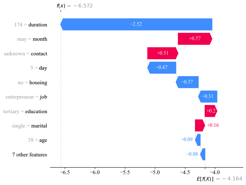
Figure 1: Local interpretation of TDS prediction using waterfall plot.

In addition, since the categorical features had undergone one-hot encoding during the data preprocessing stage, the final features only take values of 0 or 1, which may affect the clarity of the waterfall plot. Therefore, we mapped the encoded features back to their original categories and aggregated the SHAP value accordingly.

Specifically, duration had the largest negative contributions to this customer’s subscription, with the SHAP value of -2.52. It is followed by the day, housing and job, corresponding to SHAP values of -0.47, -0.37 and -0.31. Nevertheless, month and contact were the top two positive contributors, with the SHAP values of +0.57 and +0.51. This visualization clarifies how specific feature values impact the model’s prediction for a given customer.

4.2.2. Global interpretation

A SHAP feature importance plot was employed to obtain a global comprehension of the factors influencing the CatBoost model’s prediction. Unlike traditional feature importance calculations, this bar chart ranks the features based on their overall importance, measured by their mean absolute SHAP values across all the given samples. This ranking provides a clear picture of which features contribute most to the model's predictions.

Similar to section 4.2.1, the categorical features were one-hot encoded during preprocessing, which may reduce the clarity of the feature importance plot. To address this problem, we mapped the encoded features back to their original categories and aggregated the mean absolute SHAP values accordingly.

As depicted in Figure 2, the duration holds the highest importance, with a value of 1.54, which means this feature plays a key role in determining the likelihood of a customer’s subscription to a term deposit. After this, contact and month also influence the outcome considerably, with the mean absolute SHAP values of 0.66 and 0.52. In contrast, features like previous, pdays and default demonstrate the values of less than 0.1, indicating that these factors have a relatively less impact on the prediction results.

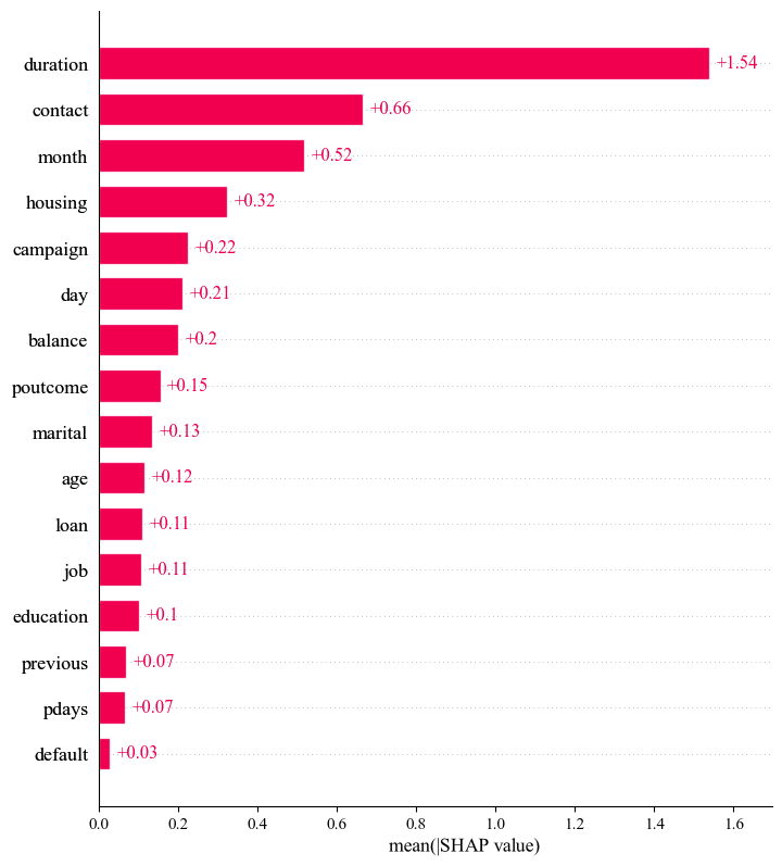
Figure 2: Global interpretation of TDS prediction using feature importance plot.

In general, the interpretability analysis based on SHAP provides insights into each feature’s local and global importance, enhancing the model’s transparency and offering guidance for improving model performance and refining feature selection.

5. Conclusion

This paper aims to provide valuable insights into the bank term deposit subscription prediction based on the state-of-the-art integrated tree model, CatBoost, and the SHAP interpretability method. Among the selected nine ML models, CatBoost presented the superior performance, which was further optimized through grid search. In addition, integrating global and local interpretations based on SHAP offered an in-depth understanding of the each feature’s contribution and the model’s decision-making process. Future research should explore the potential of other advanced methods and their application in real-word scenarios.

References

[1]. H. Abbasimehr and M. Shabani, "A new methodology for customer behavior analysis using time series clustering: A case study on a bank’s customers, " Kybernetes, vol. 50, no. 2, pp. 221-242, 2021.
[2]. V. Ivashina and D. Scharfstein, "Bank lending during the financial crisis of 2008, " Journal of Financial economics, vol. 97, no. 3, pp. 319-338, 2010.
[3]. Y. Feng, Y. Yin, D. Wang, and L. Dhamotharan, "A dynamic ensemble selection method for bank telemarketing sales prediction, " Journal of Business Research, vol. 139, pp. 368-382, 2022.
[4]. N. Ghatasheh, H. Faris, I. AlTaharwa, Y. Harb, and A. Harb, "Business analytics in telemarketing: Cost-sensitive analysis of bank campaigns using artificial neural networks, " Applied Sciences, vol. 10, no. 7, p. 2581, 2020.
[5]. X.-Y. Lu, X.-Q. Chu, M.-H. Chen, P.-C. Chang, and S.-H. Chen, "Artificial immune network with feature selection for bank term deposit recommendation, " Journal of Intelligent Information Systems, vol. 47, pp. 267-285, 2016.
[6]. C. Yan, M. Li, and W. Liu, "Prediction of bank telephone marketing results based on improved whale algorithms optimizing S_Kohonen network, " Applied Soft Computing, vol. 92, p. 106259, 2020.
[7]. M. Scott and L. Su-In, "A unified approach to interpreting model predictions, " Advances in neural information processing systems, vol. 30, pp. 4765-4774, 2017.
[8]. T. Miller, "Explanation in artificial intelligence: Insights from the social sciences, " Artificial intelligence, vol. 267, pp. 1-38, 2019.
[9]. C. Calvo-Porral and J.-P. Lévy-Mangin, "An emotion-based segmentation of bank service customers, " International Journal of Bank Marketing, vol. 38, no. 7, pp. 1441-1463, 2020.
[10]. P. Pławiak, M. Abdar, J. Pławiak, V. Makarenkov, and U. R. Acharya, "DGHNL: A new deep genetic hierarchical network of learners for prediction of credit scoring, " Information sciences, vol. 516, pp. 401-418, 2020.
[11]. E. Dumitrescu, S. Hué, C. Hurlin, and S. Tokpavi, "Machine learning for credit scoring: Improving logistic regression with non-linear decision-tree effects, " European Journal of Operational Research, vol. 297, no. 3, pp. 1178-1192, 2022.
[12]. R. A. de Lima Lemos, T. C. Silva, and B. M. Tabak, "Propension to customer churn in a financial institution: A machine learning approach, " Neural Computing and Applications, vol. 34, no. 14, pp. 11751-11768, 2022.
[13]. D. V. Carvalho, E. M. Pereira, and J. S. Cardoso, "Machine learning interpretability: A survey on methods and metrics, " Electronics, vol. 8, no. 8, p. 832, 2019.
[14]. F. Doshi-Velez and B. Kim, "Towards a rigorous science of interpretable machine learning, " arXiv preprint arXiv:1702.08608, 2017.
[15]. M. T. Ribeiro, S. Singh, and C. Guestrin, "" Why should i trust you?" Explaining the predictions of any classifier, " in Proceedings of the 22nd ACM SIGKDD international conference on knowledge discovery and data mining, 2016, pp. 1135-1144.
[16]. J. R. Quinlan, "Induction of decision trees, " Machine learning, vol. 1, pp. 81-106, 1986.
[17]. J. H. F. L. Breiman, R.A. Olshen, C.J. Stone, Classification and regression trees. Belmont: Wadsworth, 1984.
[18]. J. R. Quinlan, C4.5: programs for machine learning. Morgan Kaufmann Publishers, 1993.
[19]. K. A. Nguyen, W. Chen, B.-S. Lin, and U. Seeboonruang, "Comparison of ensemble machine learning methods for soil erosion pin measurements, " ISPRS International Journal of Geo-Information, vol. 10, no. 1, p. 42, 2021.
[20]. L. Breiman, "Bagging predictors, " Machine learning, vol. 24, pp. 123-140, 1996.
[21]. I. D. Mienye and Y. Sun, "A survey of ensemble learning: Concepts, algorithms, applications, and prospects, " IEEE Access, vol. 10, pp. 99129-99149, 2022.
[22]. L. Breiman, "Random forests, " Machine learning, vol. 45, pp. 5-32, 2001.
[23]. P. Geurts, D. Ernst, and L. Wehenkel, "Extremely randomized trees, " Machine learning, vol. 63, pp. 3-42, 2006.
[24]. Y. Freund and R. E. Schapire, "A decision-theoretic generalization of on-line learning and an application to boosting, " Journal of computer and system sciences, vol. 55, no. 1, pp. 119-139, 1997.
[25]. J. H. Friedman, "Greedy function approximation: a gradient boosting machine, " Annals of statistics, pp. 1189-1232, 2001.
[26]. T. Chen and C. Guestrin, "Xgboost: A scalable tree boosting system, " in Proceedings of the 22nd acm sigkdd international conference on knowledge discovery and data mining, 2016, pp. 785-794.
[27]. G. Ke et al., "Lightgbm: A highly efficient gradient boosting decision tree, " Advances in neural information processing systems, vol. 30, 2017.
[28]. L. Prokhorenkova, G. Gusev, A. Vorobev, A. V. Dorogush, and A. Gulin, "CatBoost: unbiased boosting with categorical features, " Advances in neural information processing systems, vol. 31, 2018.
[29]. L. S. Shapley, "17. A Value for n-Person Games, " in Contributions to the Theory of Games, Volume II, K. Harold William and T. Albert William, Eds. Princeton: Princeton University Press, 1953, pp. 307-318.
[30]. S. Ponnarasu. (2024). Bank Marketing: Term Deposits Classification. Retrieved from https://www.kaggle.com/datasets/saranyaponnarasu/bank-marketing-term-deposits-classification/data
Cite this article
Yu,Q. (2025). Enhancing Bank Term Deposit Predictions: A Machine Learning Approach with CatBoost and SHAP. Applied and Computational Engineering,120,171-180.
Data availability
The datasets used and/or analyzed during the current study will be available from the authors upon reasonable request.
Disclaimer/Publisher's Note
The statements, opinions and data contained in all publications are solely those of the individual author(s) and contributor(s) and not of EWA Publishing and/or the editor(s). EWA Publishing and/or the editor(s) disclaim responsibility for any injury to people or property resulting from any ideas, methods, instructions or products referred to in the content.
About volume
Volume title: Proceedings of the 5th International Conference on Signal Processing and Machine Learning
© 2024 by the author(s). Licensee EWA Publishing, Oxford, UK. This article is an open access article distributed under the terms and
conditions of the Creative Commons Attribution (CC BY) license. Authors who
publish this series agree to the following terms:
1. Authors retain copyright and grant the series right of first publication with the work simultaneously licensed under a Creative Commons
Attribution License that allows others to share the work with an acknowledgment of the work's authorship and initial publication in this
series.
2. Authors are able to enter into separate, additional contractual arrangements for the non-exclusive distribution of the series's published
version of the work (e.g., post it to an institutional repository or publish it in a book), with an acknowledgment of its initial
publication in this series.
3. Authors are permitted and encouraged to post their work online (e.g., in institutional repositories or on their website) prior to and
during the submission process, as it can lead to productive exchanges, as well as earlier and greater citation of published work (See
Open access policy for details).