1. Introduction

With the development of event-triggered control theory, it finds broad application across different communication scenarios, such as Multi-Agent Systems [1] and switched systems [2]. On the one hand, it effectively improves communication efficiency; but on the other hand, it has limitations. Traditional event control methods often struggle to utilize event transmission effectively when communication resources are limited, resulting in constrained savings in communication bandwidth. In practice, AET control methods based on model predictive control offer promising solutions to these issues [3]. However, when selecting trigger condition thresholds, it is important to consider how to increase the rate of change in the initial state while slowing it down as stability is approached. Therefore, we propose an AET control method based on a sampling error system.

The control schemes presented in [4,5] are static and lack the capability to dynamically adjust triggering constraints. In contrast, the AET control method proposed in this paper has several advantages: it can adaptively adjust trigger constraints, dynamically respond to sampling errors, fully exploit the benefits of event triggering under limited communication resources, and maintain expected control performance while conserving more communication bandwidth. Compared to [6], the threshold constraint condition presented in this paper can reach and converge to a stable state faster, minimizing the volume of sampled data that must be transmitted. Furthermore, this paper’s primary contributions are as follows:

1) This study introduces a new AET control approach grounded in the sampling error system. Unlike the methods presented in [4][5], the proposed adaptive trigger control method effectively maintains the advantages of event- triggered under limited communication resources, allowing for greater savings in communication bandwidth. Furthermore, it guarantees expected control performance while reducing transmission data.

2) The trigger conditions are further optimized compared to [6], enabling faster convergence to a stable state and minimizing the amount of data that needs to be transmitted.

Within this work, R signifies the set of real numbers, Rⁿ is space of real n-dimensional vector, R^m is space of real m-dimensional vector, \( {L_{2}} \) represents space of signals: \( {L_{2}}=\lbrace ‖a(k)||2 \lt ∞\rbrace , N \) stands for the set of natural numbers, \( ‖a(k)||2 \) refers to \( a(k)∈{R^{n}}: \sqrt[]{\sum _{k=0}^{ ∞}{||a(k)||^{2}}} \) .

The organization of this paper is detailed below. Section II covers the system dynamics, assumptions, lemmas, and problem formulation. Section III outlines the main findings, encompassing the AET method, controller design, stability analysis, and solutions for gain parameters. Section IV provides the conclusion of the paper.

2. Foundations and Problem Statement

This section provides the system’s dynamic description, relevant assumptions and lemmas, as well as the problem formulation.

2.1. System Dynamics

Considering the sampled data error, the state space model expression of the system is given by

\( \begin{cases} \begin{array}{c} x(t) =Ax(t)+B(t)+{B_{1}}ω(t), \\ y(t) =Cx(t), \end{array} \end{cases} \) (1)

where \( x(t)∈{R^{n}} \) and \( u(t)∈{R^{m}} \) are state control vectors and control input vectors \( , ω∈{L_{2}}[0, ∞) \) is an external perturbation. The matrices \( A, B,{ and B_{1}} \) are all constant coefficients matrices, each having appropriate dimensions. The system’s initial state is given as \( x (0) = 0 \) .

In this article, the controller’s computational delay and the delay during the transmission from the controller to the actuator are neglected.

Here, some necessary assumptions and lemma are given.

Assumption 1

The sensors are activated by time, with system states sampled at a fixed interval h>0, and all transmitted packets are provided with timestamps.

Assumption 2

Data transmission is determined by an event-triggered scheme. Upon the acquisition of the control data, it dispatches a timestamp synchronized with the measured value into the control loop.

Assumption 3

A zero-order holder (ZOH) generates the control input of the system. When the latest control input has not been received, ZOH is employed to maintain the current control input state. The holding time \( t∈Ω \) is defined as \( [{t_{k}}h+{η_{1}}, {t_{k+1}}h+{η_{1}}] \) , where \( { η_{1}} \) is the stable transmission time-delay existing from the sensor to the controller.

Lemma 1 [7]:

Take into account the following system where

\( \begin{cases} \begin{array}{c} \dot{x}(t) =Ax (t)+{A_{1}}x(t-τ(t))+{B_{1}}ω(t), \\ z(t)={C_{0}}x(t)+{C_{1}}x(t-τ(t)), \\ t∈[{t_{k}},{t_{k+1}}), τ(t)=t-{t_{k}}. \end{array} \end{cases} \)

Here, \( x(t)∈{R^{n}} \) represents the state vector, \( ω(t)∈ {R^{{n_{ω}}}} \) represents the disturbance, and \( z(t)∈ {R^{{n_{z}}}} \) is the controlled output. Matrices A, \( {A_{1}},{ B_{1}},{ C_{0}} \) and \( { C_{1}} \) have constant values with appropriate dimensions. Admit conditions that \( \dot{\bar{V}}(t)+{z^{T}}(t)z(t)-{γ^{2}}{ω^{T}}(t)ω(t) \lt 0 \) , where \( \bar{V}(t)=V(t,{x_{t,}}{\dot{x}_{t}}) \) . Almost for all t, \( ∀ ω ≠ 0 \) and a prescribed γ > 0, then the following results hold. For every nonzero \( ω∈{L_{2}}[0, ∞) \) and under the zero initial condition, \( J = \) \( \int _{0}^{∞}[{β^{2}}{x^{T}}(s)x(s)-{γ^{2}}{ω^{T}}(s)ω(s)]ds \) < 0.

2.2. Problem Formulation

For given scalars \( γ \gt 0 \) and \( β \gt 0 \) , set the performance index J to be:

\( J = \) \( \int _{0}^{∞}[{β^{2}}{x^{T}}(s)x(s)-{γ^{2}}{ω^{T}}(s)ω(s)]ds \) . (2)

We devise an event-triggered state feedback control law in the format of form: \( u(t)=Kx({t_{k}}h), t∈ Ω \) ensuring that the corresponding closed-loop system attains internal asymptotic stability. and \( J \lt 0 \) for the initial condition \( { x_{0}}= 0 \) and all nonzero \( ω∈{L_{2}}[0, ∞). \)

As can be seen from the expression in (8), a portion of sampled data stays untransmitted during the intervals between two transmission instances. With the aim of incorporating the event-triggered transmission scheme to determine the necessity of transmitting the current sampled data, an effective approach is presented. This approach considers the error of the sampled data at each sampling moment, resulting in the division of the ZOH holding interval \( Ω \) into subintervals.

\( {Ω_{n, k}}=[{t_{k}}h+ nh +{η_{1}} ,{t_{k}}h +nh+{η_{1}}+h) i.e. Ω=∪{Ω_{n, k}} \) , \( n = 0,1…{t_{k+1}}-{t_{k}}-1 \) .

Define

\( η(t) ≜ t - {m_{n, k}}h, t∈{ Ω_{n, k}} \) (3)

\( e({m_{n, k}}h) ≜ x({m_{n, k}}h)-x({t_{k}}h) \) (4)

with \( {m_{n, k}}h= {t_{k}}h +nh, n=0,1,2…,{t_{k+1}}-{t_{k}}-1 \) .

In light of the meaning of  \( η(t) \) , it turns out to be a piecewise linear function satisfying the following conditions.

\( \dot{η}(t)=1, {η_{1}}≤ h+ η(t) ≤ {η_{2}}, t∈{ Ω_{n ,k}} and t ≠{ m_{n, k}}+{η_{1}}. \) (5)

Then the control law is represented as

\( u(t)=K[x(t-η(t))-e(t-η(t)], t∈{ Ω_{n, k}} \) (6)

From (1) and (6), the sampled-data error dependent system is of the following form.

\( \dot{x}=Ax(t)+ BKx(t-η(t))- BKe({m_{n, k}}h)+{B_{1}}ω(t), t∈{Ω_{n, k}}. \) (7)

Remark 1: By the definition of \( η(t) \) and \( e{(m_{n, k}}h) \) , it can be noted that the calculation \( e{(m_{n,k}}h) \) occurs solely at the sampling instant \( { t_{k}}h+ nh \) . Thereby, it’s not essential to conduct continuous measurement.

Remark 2: Model (7) notably includes a specific case where \( {η_{1}}= 0 \) . From equation (5), it is evident that \( {η_{2}} \) is influenced by the sampling period as well as the transmission delay. When \( {η_{2}} \) is determined, it serves the purpose of balancing the sampling period with the permissible transmission delay.

The primary initiatives carried out in this paper are enumerated below.

1) Propose an AET mechanism framework and conduct a stability analysis of the designed controller.

2) Provide the LMI method for solving the controller gain parameters.

3. Main Results

3.1. Adaptive Event-Triggered Mechanism

Assuming that data transmission depends on predefined conditions rather than occurring at fixed time intervals, this approach determines the timing of the next data transmission. In each control cycle, the sampled data is transmitted conditionally by an AET generator, while the control quantity is continuously adjusted by the model predictive controller. Compared to the schemes proposed in [4][5], the main advantage of the suggested AET predictive control scheme shown in Fig.1 is its ability to dynamically adjust the threshold. The increment is faster at the initial moment, allowing the system to converge more quickly as it approaches the steady state. Building on this description, the adaptive event generator determines the next transmission time as

\( {t_{k+1}}h= {t_{k}}h+{min_{n∈N}}\lbrace {e^{T}}({i_{k}}h)Φe({i_{k}}h) \gt σ({t_{k}}h){x^{T}}({t_{k}}h)Φx({t_{k}}h)\rbrace \) (8)

where \( Φ \gt 0 \) stands for the weight coefficient matrix, h denotes the system sampling period, \( {t_{k}}(k = 0,1,2…) \) are some integers such that \( \lbrace {t_{0}},{t_{1}},{t_{2}}…\rbrace ⊂\lbrace 0,1,2…\rbrace ; e({i_{k}}h) \) represents the current sampling moment data \( x({i_{k}}h) \) and the latest transmission data \( x({t_{k}}h) \) , that is

\( e({i_{k}}h) ≜ x({i_{k}}h)-x({t_{k}}h),{ i_{k}}h∈({t_{k}}h,{t_{k+1}}h]. \) (9)

Moreover, \( σ({t_{k}}h) \) in (8) is governed by the following adaptive rule.

\( σ({t_{k+1}}h)=max\lbrace \underset{λ}{\underbrace{1-αtanh{[β(||x({t_{k+1}}h)||-||x({t_{k}}h)||)]}}},{ σ_{m}}\rbrace \) (10)

where \( tanh{(∙)} \) represents the hyperbolic tangent function, 0 < α and 0 < β are given constants to adjust the output of \( tanh{(∙)},{ σ_{m}} \) is the predefined lower bound of \( σ({t_{k}}h). In this research, we have σ(0)={σ_{m}}. \)

The transmission events are influenced by the error \( e({i_{k}}h) \) , the latest transmitted states \( x({t_{k}}h) \) , and the adjustable threshold \( σ({t_{k}}h) \) .

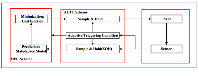
Figure 1: Structural diagram of proposed AET-MPC

Figure 2 provides an example illustrating the core concept of the proposed scheme, where \( {t_{k}}h \) represents the triggered transmission instants. Clearly, not all data will be transmitted, but only the data that meets the constraint conditions will be transmitted. For instance, the data at time 0, h, 3h, 6h and 9h are transmitted, while the data at the rest of times remain untransmitted.

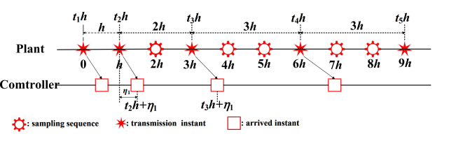
Figure 2: Specific instance of the time evolution of the sampling and transmission sequences.

Note that the function \( tanh{(∙)} \) has both an upper and lower bound, denoted as \( tanh{(∙)}∈ (-1,1) \) . This paper leverages these properties to dynamically adjust the threshold \( σ({t_{k}}h). \) For example, when \( ‖x({t_{k+1}}h)‖ \gt ‖x({t_{k}}h)‖, \) we can achieve \( 0 \lt λ \lt 1 and σ({t_{k+1}}h) \lt σ({t_{k}}h), \) which means using a smaller \( σ({t_{k+1}}h) \) to establish a faster communication frequency, thereby reducing the error between \( ‖x({t_{k+1}}h)‖ \) and \( ‖x({t_{k}}h)‖. \) Conversely, by setting a slower communication frequency \( σ({t_{k+1}}h), \) more communication bandwidth can be conserved.

Remak 3: The event-triggered threshold \( σ \) is a pre-selected constant, and the parameters \( σ({t_{k}}h) \) can be dynamically adjusted according to the adaptive rules (10), depending on the current \( x({t_{k+1}}h), \) latest transmission data \( x({t_{k}}h), α, β \) and the simultaneous adjustment \( { σ_{m}} \) . In addition, if \( { σ_{m}} \) is sufficiently close to zero, this implies that \( {t_{k+1}}={t_{k}}h +h \) and all sampled data are transmitted with a constant sampling period h. In this case, the proposed adaptive communication scheme will degenerate into the general scheme [8][9]. More generally, if \( α ≡ 0 \) , the scheme will degenerate into the constant communication scheme [10][11].

3.2. System Stability Analysis and Parameter Solving

This subsection attaches importance to analyzing the system’s stability and providing ways to determine the parameters in event-triggered solution schemes.

Consequently, focus on the ensuing Lyapunov function.

\( V(t,{x_{t}})={V_{1}}(t,{x_{t}})+{V_{2}}(t,{x_{t}}), t∈{ Ω_{n ,k}}, \) (11)

where \( {x_{t}}=x (t+θ), ∀θ∈[-{η_{2}},0] \) . Then, one gets

\( {V_{1}}(t,{x_{t}}) = {x^{T}}(t)Px(t)+\int _{t-{η_{2}}}^{t-{η_{1}}}\int _{s}^{t}{\dot{x}^{T}}(ο){S_{2}}\dot{x}(ο)dοds+ {η_{1}}\int _{t-{η_{1}}}^{t}\int _{s}^{t}{\dot{x}^{T}}(ο){S_{1}}\dot{x}(ν)dοds+\sum _{i=1}^{2}\int _{t-{η_{i}}}^{t}{x^{T}}(ο){P_{i}}x(ο)dο \) ,

where \( P \gt 0,{ P_{i}} \gt 0,{ S_{i}} \gt 0(i =1, 2) \) and

\( {V_{2}}(t,{x_{t}}) = ({η_{2}}-η(t))[{ς^{T}}(t)\hat{R}ς(t)+\int _{t-κ}^{t}{\dot{x}^{T}}(ο){S_{3}}\dot{x}(ο)dο] \) .

with

\( {ς^{T}}(t) = [{ x^{T}}(t),{ x^{T}}(t-κ)], κ = η(t)-{η_{1}} \) .

\( \hat{R}=[\begin{matrix}{R_{1}} & {R_{2}}-{R_{1}} \\ * & {R_{1}}-R_{2}^{T}-{R_{2}} \\ \end{matrix}], {S_{3}} \gt 0, {R_{1}} \gt 0 \) and \( {R_{2}} \) being chosen such that \( V(t,{x_{t}}) ≥ 0 \) .

In what follows, the forms of \( {V_{1}} \) and V₂ will be utilized to determine whether the system is stable.

Theorem 1: For given some constants γ >0, β >0, σ > 0, η₁>0, h>0 and a matrix K under an event-triggered transmission scheme (8), the system (7) from ω to x is finite-gain L₂-stable with gain less than γ/β. If positive matrices P, R₁, Φ, P₁, P₂, S_i and appropriately sized matrices R₂ and L_i​ (i =1,2,3) exist, and the conditions to follow are met.

\( [\begin{matrix}{P_{1}} + h{R_{1}} & * \\ hR_{2}^{T}-h{R_{1}} & h{R_{1}}-hR_{2}^{T}-h{R_{2}} \\ \end{matrix}] \gt 0. \) (12)

\( [\begin{matrix}Ε+ψ+{ψ^{T}}+(1-ρ)hΣ & * \\ F_{21}^{ρ} & -{F_{22}} \\ \end{matrix}] \lt 0, ρ = 0,1 \) (13)

with

\( Ε = diag\lbrace {P_{1}}+{P_{2}}-{R_{1}}+{β^{2}}I, -{P_{1}},0, -{P_{2}}, -{γ^{2}}I, R_{2}^{T}+{R_{2}}-{R_{1}}\rbrace +2P{I_{1}}{I_{2}}+σ{I_{4}}ΦI_{4}^{T}-{S_{1}}{I_{5}}I_{5}^{T}+2{I_{1}}({R_{1}}-{R_{2}})I_{3}^{T} \) ,

\( F_{21}^{ ρ}= col\lbrace {η_{1}}{S_{1}}{I_{2}}, h{S_{2}}{I_{2}}, hL_{ρ+1}^{T}h{S_{3}}{I_{2}}+ρhL_{3}^{T}\rbrace , \)

\( {F_{22}}= diag\lbrace {S_{1}}, h{S_{2}}, h{S_{2}}, h{S_{3}}\rbrace \) ,

\( ψ = [{L_{3}} {L_{2}} {L_{1}}-{L_{2}} 0 -{L_{1}} -{L_{3}} 0] \) ,

\( Σ = 2{I_{1}}{R_{1}}{I_{2}}+2{I_{3}}(R_{2}^{T}-R_{1}^{T}){I_{2}} \) ,

where

\( {I_{1}}={[I 0 0 0 0 0 0]^{T}} \) ,

\( {I_{2}}=[A 0 BK -BK 0 {B_{1}} 0] \) ,

\( {I_{3}}={[0 0 0 0 0 0 I]^{T}}, \)

\( {I_{4}}={[0 0 I -I 0 0 0]^{T}} \) ,

\( {I_{5}}={[I -I 0 0 0 0 0]^{T}} \) .

Proof: When the time derivative of \( V(t,{x_{t}}) \) in (11) is computed along the trajectory of system (7), it leads to

\( \dot{V}(t,{x_{t}}) = 2{x^{T}}(t)P\dot{x}(t)-\int _{t-κ}^{t}{\dot{x}^{T}}(ο){S_{3}}\dot{x}(ο)dο - {ς^{T}}(t)\hat{R}ς(t)+η_{1}^{2}{\dot{x}^{T}}(t){S_{1}}\dot{x}(t)-{η_{1}}\int _{t-κ}^{t}{\dot{x}^{T}}(ο){S_{3}}\dot{x}(ο)dο+h{\dot{x}^{T}}(t){S_{2}}\dot{x}(t) \)

\( -\int _{t-{η_{2}}}^{t-{η_{1}}}{\dot{x}^{T}}(s){S_{2}}\dot{x}(s)ds+({η_{2}}-η(t))\lbrace {2ς^{T}}(t)\hat{R}{[{\dot{x}^{T}}(t), 0]^{T}}+{\dot{x}^{T}}(t){S_{3}}\dot{x}(t)\rbrace +\sum _{i =1}^{2}[{x^{T}}(t){P_{i}}x(t)-{x^{T}}(t-{η_{i}}){P_{i}}x(t-{η_{i}})] \) ,

\( t∈{Ω_{n,k}} \) . (14)

From (10), it is clear that the minimum value of \( σ ({m_{n, k}}h) \) is \( { σ_{m}} \) . If the currently sampled data isn’t transmitted, the following relationship holds.

\( {e^{T}}({m_{n, k}}h)Φe({m_{n, k}}h) \lt {σ_{m}}{x^{T}}({t_{k}}h)Φx({t_{k}}h)={σ_{m}}{(x(t-η(t))-e({m_{n,k}}h))^{T}}Φ(x(t-η(t))-e({m_{n,k}}h)), t∈{Ω_{n, k}} \) (15)

By applying the Newton-Leibniz formula and introducing matrices \( {L_{i}} \) ( i =1, 2, 3) of suitable dimensions to handle the integral terms in (14), the following result is derived from equations (14) and (15).

\( \dot{V}(t,{x_{t}}) \lt {ξ^{T}}(t){Δ_{0}}ξ(t)-{β^{2}}{x^{T}}(t)+{γ^{2}}{ω^{T}}(t)ω(t). \) (16)

with

\( {ξ^{T}}(t)=[{ x^{T}}(t), { x^{T}}(t-{η_{1}}),{ x^{T}}(t-η(t)), {e^{T}}({m_{n, k}}h),{ x^{T}}(t-{η_{1}}), { ω^{T}}(t),{ x^{T}}(t-κ)] \) ,

\( {Δ_{0}}= Ε+({η_{2}}-η(t)){Δ_{1}}+(η(t)-{η_{1}}){Δ_{2}}+ψ+{ψ^{T}}+η_{1}^{2}I_{2}^{T}{S_{1}}{I_{2}}+hI_{2}^{T}{S_{2}}{I_{2}} \) ,

\( {Δ_{1}}={ L_{1}}S_{2}^{ -1}L_{1}^{T}+I_{2}^{T}{S_{3}}{I_{2}}+Σ \) ,

\( {Δ_{2}}={ L_{2}}S_{2}^{ -1}L_{2}^{T}+I_{2}^{T}{S_{3}}{I_{2}}+Σ \) ,

where \( Ε, ψ,{ I_{2}} \) and \( Σ \) are defined in Theorem 1. □

Through the Lyapunov function in (11) and equations (13) to (16), it can be concluded that system (7) with \( ω(t)=0 \) is asymptotically stable under zero initial conditions. Furthermore, this result is supported by (12). Applying Lemma 1, the system is shown to be L₂ finite gain stable with the gain constrained by \( γ / β \) .

Theorem 2: Given some constants γ>0, β>0, σ >0, η₁>0 and h>0 under the event-triggered transmission scheme (8), the system (7) remains finite-gain stable from \( ω \) to x with a gain less than γ / β , and the state feedback controller gain is expressed as \( K=Y{X^{ -1}} \) , if there exist positive matrices \( X, {\widetilde{R}_{1}}, \widetilde{Φ }, {\widetilde{P}_{i}}, {\widetilde{S}_{i}} \) and a scalar \( λ \gt 0, \) and suitable dimensioned matrices \( {\widetilde{R}_{2}} \gt 0 \) and \( {\widetilde{L}_{i}} \gt 0 ( i = 1, 2, 3), \) in a way that the conditions outlined are fulfilled.

\( [\begin{matrix}X+h{\widetilde{R}_{1}} & * \\ h\widetilde{R}_{2}^{T}-h{\widetilde{R}_{1}} & h{\widetilde{R}_{1}}-h\widetilde{R}_{2}^{T}-h{\widetilde{R}_{2}} \\ \end{matrix}] \gt 0 \) ,(17)

\( [\begin{matrix}\widetilde{E}+\widetilde{ψ}+{\widetilde{ψ}^{T}} & * \\ \widetilde{F}_{21}^{ ρ} & -\widetilde{F}_{22}^{ ρ } \\ \end{matrix}] \lt 0, ρ= 0, 1, \) (18)

where

\( \widetilde{E} = diag\lbrace {\widetilde{P}_{1}}+{\widetilde{P}_{2}}-{\widetilde{R}_{1}}, 0, -\widetilde{Φ}, {\widetilde{P}_{2}} , -{γ^{2}}I, \widetilde{R}_{2}^{T}+{\widetilde{R}_{2}}-{\widetilde{R}_{1}}\rbrace -{\widetilde{S}_{1}}{I_{5}}I_{5}^{T}+2{I_{1}}{\widetilde{I}_{2}}+2{I_{1}}({\widetilde{R}_{1}}-{\widetilde{R}_{2}})I_{3}^{T}+σ{I_{4}}\widetilde{Φ}I_{4}^{T} \) ,

\( \widetilde{F}_{21}^{ 0} = col\lbrace {η_{1}}{\widetilde{I}_{2}}, \sqrt[]{h}{\widetilde{I}_{2}}, \sqrt[]{h}\widetilde{L}_{1}^{T}, \sqrt[]{h}{\widetilde{I}_{2}}, \sqrt[]{2}{\widetilde{I}_{2}},h{\widetilde{R}_{1}}I_{1}^{T},h({\widetilde{R}_{2}}-{\widetilde{R}_{1}})I_{3}^{T}, βX\rbrace , \)

\( \widetilde{F}_{22}^{0} = diag\lbrace X\widetilde{S}_{1}^{-1}X, X\widetilde{S}_{2}^{-1}X, X\widetilde{S}_{3}^{-1}X, X{λ^{-1}}X, λI, λI, I\rbrace , \)

\( \widetilde{F}_{21}^{1} = col\lbrace {η_{1}}{\widetilde{I}_{2}}, h{\widetilde{I}_{2}}, h\widetilde{L}_{2}^{T}, h\widetilde{L}_{3}^{T}\rbrace , \)

\( \widetilde{F}_{22}^{1} = diag\lbrace X\widetilde{S}_{1}^{-1}X, hX\widetilde{S}_{2}^{-1}X, h{\widetilde{S}_{2}}, h{\widetilde{S}_{3}}\rbrace , \)

\( \widetilde{ψ} = [{\widetilde{L}_{3}} {\widetilde{L}_{2}} {\widetilde{L}_{1}}-{\widetilde{L}_{2}} 0 -{\widetilde{L}_{1}} -{\widetilde{L}_{3}} 0], \)

\( {\widetilde{I}_{2}} = [AX 0 BY -BY 0 {B_{1}} 0 ]. \)

Proof: Define \( X={P^{-1}} \) , \( XΦX=\widetilde{Φ} \) , \( X{P_{i}}X={\widetilde{P}_{i}}, \) \( X{\widetilde{R}_{i}}X ={\widetilde{ R}_{i}} \) (i = 1, 2), \( X{S_{j}}X={\widetilde{S}_{j}} \) , \( X{L_{j}}X={\widetilde{L}_{j}} \) ( j =1, 2, 3) and \( Y=KX \) . For any scalar \( λ \gt 0 \) , it yields

\( Σ ≤ { h^{2}}{I_{1}}{R_{1}}λ{R_{1}}I_{1}^{T}+2{I_{2}}{λ^{-1}}{I_{2}}+{h^{2}}{I_{3}}{R^{T}}{λ^{-1}}RI_{3}^{T} \) (19)

where \( R = {R_{2}}-{R_{1}} \) . Then multiply both sides of (12) with \( diag(X, X ) \) . For \( ρ = 0, \) apply \( diag( X, X, X, X, X, X, I, X, I, I, X, I ) \) on both sides of (13) \( \) and for \( ρ = 1, \) use \( diag(X, X, X, X, X, X, I, X, I, I, X, X) \) .

Employing the Schur complement and equation (19), (17) and (18), thereby completing the proof.

Nonlinear terms \( X{\widetilde{S}_{i}}X \) and \( X{λ^{-1}}X \) render the matrix inequality (18) non-convex, preventing direct resolution via the MATLAB LMI Toolbox. To this end, a variable matrix \( M_{j}^{T} \gt 0 \) \( ( j = 1, 2, 3,4) \) is introduced as

\( X\widetilde{S}_{ i}^{ -1}X ≥ {M_{i}}, X{λ^{-1}}X ≥{ M_{4}} \) (20)

Let \( { N_{j}}=M_{j}^{ -1}, {Z_{4+i}}=\widetilde{S}_{i}^{ -1}( i=1, 2, 3),{ N_{8}}={λ^{-1}}I \) and \( { N_{9}} ={ X ^{-1}} \) . Then (18) can be replaced by

\( [\begin{matrix}{N_{i}} & {N_{9}} \\ * & {N_{4+i}} \\ \end{matrix}]≥0, i =1, 2, 3, 4. \) (21)

Thus, it becomes possible to subsequently transform the original non-convex minimization problem into a minimization problem constrained by LMI conditions.

\( \begin{cases} \begin{array}{c} min tr (\sum _{j=1}^{4}{N_{j}}{M_{j}}+\sum _{i=1}^{3}{N_{4+i}}{\widetilde{S}_{i}}+{N_{8}}λI) \\ subject to:(17),G, (21) and \\ [\begin{matrix}{M_{j}} & I \\ * & {Z_{j}} \\ \end{matrix}]≥ 0, [\begin{matrix}X & I \\ * & {N_{9}} \\ \end{matrix}]≥ 0, \\ [\begin{matrix}{\widetilde{S}_{i}} & I \\ * & {N_{4+i}} \\ \end{matrix}]≥ 0, [\begin{matrix}λI & I \\ * & {N_{8}} \\ \end{matrix}]≥ 0, \end{array} \end{cases} \) (22)

where G is obtained from (18) by substituting \( X {\widetilde{S}_{i }}X \) and \( X {λ^{-1}}X \) with \( {M_{j}} \) and \( { M_{4}} \) in (22), respectively. The minimization problem discussed is solvable using CCL [12].

To derive a practical solution, the following algorithm is introduced to systematically identify the optimal parameters \( h, σ, Φ \) and K.

Define:

\( \begin{cases} \begin{array}{c} min f (σ) \\ subject to: σ∈(0, 1) \end{array} \end{cases} \) (23)

where

\( f(σ) = \frac{the quantity of the trasmitted sampled-data}{the quantity of all the sampled-data} \)

To achieve a feasible solution, the following algorithm is proposed to obtain the optimal parameters \( h, σ, Φ \) and K.

Remark 4: In this analysis, it is assumed that all system states are fully observable and can be utilized for state feedback control. If the states of the system cannot all be measured, state estimation can be performed through a sampled control system. Similarly, if \( {η_{1}}= 0 \) this can also be solved using a defined Lyapunov function (11).

Remark 5: The AET scheme proposed in this paper builds upon the static event-triggered scheme, utilizing the threshold σ from the static event-triggered scheme as the initial value for the adaptive scheme. Consequently, the selection and determination of other parameters remain consistent with those in [13].

4. Conclusion

The paper has proposed an AET control method based on a sampling error system. The AET mechanism is implemented to allow the system to dynamically modify the trigger threshold, reducing the transmitted sampling data and conserving bandwidth. Compared to traditional event-triggered mechanisms, the proposed approach has not only preserved the benefits of event-triggered control under constrained communication resources but also optimized bandwidth usage while maintaining the desired control performance. This approach has offered valuable insights for enhancing event-triggered performance and improving communication transmission efficiency.

References

[1]. Shi X, Li Y, Du C, et al. Fully distributed event-triggered control of nonlinear multi-agent systems under directed graphs: a model-free DRL approach[J]. IEEE Transactions on Automatic Control, 2024.
[2]. Zhang T, Cao J, Li X. Prescribed-time control of switched systems: an event-triggered impulsive control approach[J]. IEEE Transactions on Systems, Man, and Cybernetics: Systems, 2024.
[3]. Tang X, Zhao K, Zhang L, et al. Adaptive event-triggered output feedback control for uncertain networked T–S fuzzy system with data loss and bounded disturbance: an efficient MPC strategy[J]. Journal of the Franklin Institute, 2024.
[4]. He N, Li Y, Li H, et al. PID-based event-triggered MPC for constrained nonlinear cyber-physical systems: theory and application[J]. IEEE Transactions on Industrial Electronics, 2024.
[5]. He N, Chen Q, Xu Z, et al. An error quasi quadratic differential based event-triggered MPC for continuous perturbed nonlinear systems[J]. International Journal of Control, Automation and Systems, 2024.
[6]. Peng C, Yang M, Zhang J, et al. Network-based H∞ control for T–S fuzzy systems with an adaptive event-triggered communication scheme[J]. Fuzzy Sets and systems, 2017.
[7]. Fridman E. A refined input delay approach to sampled-data control[J]. Automatica, 2010.
[8]. Dolk V S, Scheres K J A, Postoyan R, et al. Time-and event-triggered communication for multi-agent systems–part I: general framework[J]. IEEE Transactions on Automatic Control, 2024.
[9]. Li X, Tang Y, Zou Y, et al. A hybrid time/event-triggered interaction framework for multi-agent consensus with relative measurements[J]. Automatica, 2024.
[10]. Deng L, Shu Z, Chen T. Event-triggered robust MPC with terminal inequality constraints: a data-driven approach[J]. IEEE Transactions on Automatic Control, 2024.
[11]. Liu X, Qiu L, Fang Y, et al. A two-step event-triggered-based data-driven predictive control for power converters[J]. IEEE Transactions on Industrial Electronics, 2024.
[12]. El Ghaoui L, Oustry F, AitRami M. A cone complementarity linearization algorithm for static output-feedback and related problems[J]. IEEE transactions on automatic control, 1997.
[13]. Peng C, Han Q L. A novel event-triggered transmission scheme and "L" _"2" control co-design for sampled data control systems[J]. IEEE Transactions on Automatic Control, 2013.
Cite this article
Hu,J. (2025). An Adaptive Event-Triggered Predictive Control Method. Applied and Computational Engineering,121,42-50.
Data availability
The datasets used and/or analyzed during the current study will be available from the authors upon reasonable request.
Disclaimer/Publisher's Note
The statements, opinions and data contained in all publications are solely those of the individual author(s) and contributor(s) and not of EWA Publishing and/or the editor(s). EWA Publishing and/or the editor(s) disclaim responsibility for any injury to people or property resulting from any ideas, methods, instructions or products referred to in the content.
About volume
Volume title: Proceedings of the 5th International Conference on Signal Processing and Machine Learning
© 2024 by the author(s). Licensee EWA Publishing, Oxford, UK. This article is an open access article distributed under the terms and
conditions of the Creative Commons Attribution (CC BY) license. Authors who
publish this series agree to the following terms:
1. Authors retain copyright and grant the series right of first publication with the work simultaneously licensed under a Creative Commons
Attribution License that allows others to share the work with an acknowledgment of the work's authorship and initial publication in this
series.
2. Authors are able to enter into separate, additional contractual arrangements for the non-exclusive distribution of the series's published
version of the work (e.g., post it to an institutional repository or publish it in a book), with an acknowledgment of its initial
publication in this series.
3. Authors are permitted and encouraged to post their work online (e.g., in institutional repositories or on their website) prior to and
during the submission process, as it can lead to productive exchanges, as well as earlier and greater citation of published work (See
Open access policy for details).