1.Introduction

With the rapid development of artificial intelligence, Deep Neural Networks (DNNs) have become the cornerstone of various applications, including computer vision, natural language processing, and autonomous driving. As the complexity of DNNs grows, their computational demands have surged, making the design of efficient hardware accelerators essential to achieve high performance and low energy consumption. DNN accelerators, such as Tensor Processing Units (TPUs) and custom-designed Application-Specific Integrated Circuits (ASICs), aim to address these challenges by accelerating DNN inference [1]. However, optimizing dataflow scheduling on these accelerators remains a complex issue due to the vast design space and intricate interaction between layers and hardware resources.

Traditional scheduling methods, such as heuristic-based algorithms and random search algorithms, have been widely used for DNN dataflow optimization. However, these methods often struggle with large design spaces and fail to fully adapt to the dynamic constraints of modern hardware architectures. Recent studies have explored the potential of reinforcement learning (RL) to address these challenges, enabling adaptive optimization strategies that learn from the environment to improve scheduling efficiency. RL-based approaches, such as RLMap and RELMAS, have shown promising results in optimizing DNN scheduling, outperforming conventional methods in both energy efficiency and execution time [2, 3].

This paper proposes a novel reinforcement learning framework for optimizing dataflow scheduling in DNN accelerators. This paper framework addresses the challenges of large-scale design spaces and the dynamic nature of hardware configurations. In our work, we propose a reinforcement learning framework for DNN accelerator scheduling optimization, using PPO to dynamically adjust scheduling strategies. We implement a brute-force search method for finding locally optimal solutions, ensuring that the solutions satisfy both DNN parameter constraints and hardware resource limits. We validate our approach through extensive experiments across multiple DNN models and accelerator architectures, demonstrating significant improvements in energy efficiency and execution cycles compared to existing scheduling algorithms.

In the following sections, this paper will introduce some basic theory, and detail the methodology used, the experimental setup, and the results of our comparison with state-of-the-art tools. The results confirm the effectiveness of our approach in exploring large design spaces and optimizing scheduling for different hardware configurations.

2.Basic Theory and Analysis

This section provides an overview of the essential elements involved in designing and optimizing scheduling strategies for DNN accelerators. It covers the parameters of DNN layers, the hierarchical structure of DNN accelerator components. Additionally, a review of existing scheduling optimization methods highlights their limitations and the need for a dynamic, adaptive optimization approach using reinforcement learning.

2.1.Representation of Deep Neural Networks (DNNs) and Accelerators

For designing and optimizing scheduling strategies for DNN accelerators, it is crucial to understand the parameters of DNN layers and the roles and relationships of accelerator hardware components. This section will discuss the fundamental structure of DNNs and their accelerators, to provide a foundation for constructing the scheduling optimization model and facilitate efficient dataflow scheduling.

DNNs are typically composed of multiple types of neural layers, such as convolutional layers, fully connected layers, and pooling layers, each serving distinct purposes and characterized by unique parameters [4]. However, a unified representation can be used to describe most neural layers, as illustrated in Figure 1, where eight parameters are employed,including batch Size (B), Input Channel (C), Group Size (G), Weight Width (R) and Weight Height (S), Output Channel (K), Output Width (P) and Output Height (Q). The output dimension parameters P and Q, along with the dimensions of the weight matrix, can be used to compute the size of the input feature map (U and V).

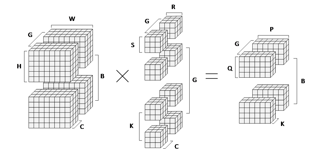
Figure 1: A unified representation of a neural layer, illustrating the meaning of each parameter.

In the computation of neural layers, three primary data types are involved: Input, which refers to the data fed into the neural layer; Weights, representing the connection weights that influence the computations within the layer; and Output, which is the result generated from processing the input data with the corresponding weights. These data types are crucial for defining the operations and interactions within neural networks.

These data types exhibit different reuse characteristics when stored and processed by the accelerator. Efficient scheduling requires careful orchestration of their movement across various levels of memory to maximize data reuse and optimize performance.

The parameters of DNN layers are associated with each other due to their shared data types. As shown in Table 1, each parameter (with the exception of G) is related to two types of data. For instance, the C is related to both input data and weight data but not to output data. These interdependencies reveal the potential for data reuse during neural network computations, which is key to optimizing performance.

Table 1: Correlations between different parameters and their associated data types.

2.2.Components of Deep Neural Network Accelerators

The primary goal of DNN accelerators is to expedite the execution of DNN inference tasks. As such, their hardware architecture typically needs to be optimized for different types of DNNs, leading to various specialized accelerator architectures [5]. This section analyzes the unified hierarchical modeling of DNN accelerator components and their role in dataflow scheduling.

As shown in Figure 2, the accelerator components can be represented in a unified hierarchical structure. Registers are typically used to store intermediate computation results or provide fast access to data, closely integrated with Multiply-Accumulate (MAC) Units. MAC units are the core of DNN computation, responsible for performing matrix multiplications and additions. Local Buffers store data transferred from global memory or higher-level caches, reducing the need to frequently access global memory and thereby lowering energy consumption. Processing Elements (PEs) are the basic units of parallel computation in DNN accelerators. Each PE usually contains multiple MAC units, registers, and local buffers. The Global Buffer facilitates data transfer between different PEs and provides cross-layer data sharing when needed. The size and bandwidth of the global buffer determine the communication capacity between PEs. In large-scale accelerators, multiple Chips can work in parallel, each containing numerous PEs, caches, and registers. Data exchange between chips is handled by a high-speed communication network. Off-chip Memory (DRAM) is used to store the parameters of the DNN model and intermediate computation results.

DNN accelerators utilize a multi-level memory hierarchy, ranging from registers and on-chip caches to off-chip memory, forming a complex storage system [6]. Register-level data access is the most efficient, but capacity is limited, while off-chip memory offers the largest capacity but incurs the highest latency and energy consumption. Therefore, during scheduling optimization, data should be reused efficiently, and frequent access to off-chip memory should be avoided whenever possible.

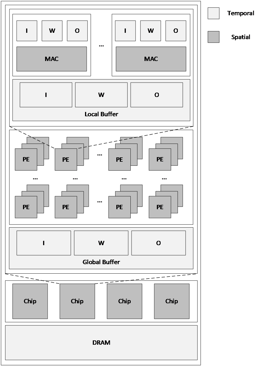
Figure 2: The hierarchical structure of DNN accelerator components and the types of data reuse.

In the multi-level hierarchy of DNN accelerators, components at different levels exhibit distinct data reuse behaviors. As shown in Fig. 2, on-chip caches achieve temporal reuse by retaining data blocks, while the spatial arrangement of MAC units, PEs, and chips enables spatial reuse of data. On-chip caches store and reuse data, enabling different dataflow modes such as Input Stationary (IS), Weight Stationary (WS), and Output Stationary (OS). These modes can coexist across various cache levels. The spatial arrangement of processing elements allows the accelerator to process multiple data blocks in parallel, thus improving computational throughput and parallelism [7]. By optimizing both spatial and temporal reuse, in combination with efficient scheduling strategies, the computational efficiency of each DNN layer can be significantly improved.

2.3.Systematic Literature Analysis

In recent years, researchers have proposed a variety of efficient solutions to address the scheduling optimization problem in DNN accelerators. These methods aim to improve the performance and energy efficiency of accelerators by optimizing dataflow scheduling and resource allocation. They explore and generate optimal scheduling strategies through different technical approaches in the complex design space.

Timeloop models various hardware architectures and simulates different dataflow scheduling strategies using its energy and execution cycle models, helping researchers find the most optimal solutions based on these metrics [8]. The evaluation model in our work is based on the framework provided by Timeloop. However, the optimization strategy used in Timeloop is essentially the random search, which makes it difficult to converge when addressing scheduling optimization problems. CoSA employs a constrained optimization approach, constructing an objective function to generate optimized scheduling schemes for DNN accelerators [9]. However, there is no guarantee that the objective function constructed by CoSA is rational and capable of guiding the solution toward an optimal result. Mind Mappings introduces a framework capable of efficiently searching the algorithm-accelerator mapping space [10]. It uses a neural network to approximate the energy and execution time of a scheduling solution. While this method can improve search efficiency, its accuracy heavily depends on the coverage of the training dataset, and we found that it was largely inaccurate in the experiments. ZigZag employs a top-down approach that performs a stepwise search through the hierarchical structure of accelerators, starting from the computation units and moving toward off-chip memory [11]. This method is inherently advantageous in generating scheduling schemes with high PE utilization, but these schedules do not necessarily guarantee optimal energy consumption or execution time. In contrast, NeuroSpector adopts a bottom-up approach, starting with off-chip memory and focusing on optimizing off-chip memory accesses, which have the greatest impact on energy consumption [12]. While it exhibits good scalability when handling large-scale neural networks, it also suffers from the inability to guarantee optimal results for the specified performance metrics.

A common limitation among current research is that most methods rely on heuristic approaches and fail to account for the varying characteristics of the scheduling optimization problem under different hardware configurations and inference tasks. A reasonable optimization method should dynamically adjust the scheduling strategy based on the specific scheduling case. In this paper, we propose a reinforcement learning-based optimization method that adjusts the optimization sequence based on the current state of the scheduling optimization, enabling adaptive optimization.

3.Methodology and Model

This chapter details our approach to optimizing dataflow scheduling on DNN accelerators. First, we define the fundamental framework of the problem, including the construction of the scheduling table and the constraint relationships. Next, we introduce the design of the reinforcement learning framework, covering the agent, environment, action space, state definition, reward function and the optimization method based on Proximal Policy Optimization (PPO). We then discuss how the use of invalid action masking. Finally, we demonstrate the brute-force search method for searching the locally optimal solutions in iterative loop.

3.1.Problem Definition

In DNN accelerators, scheduling optimization refers to minimizing energy consumption and execution time, all within the constraints of hardware and neural layer parameters. We represent the mapping relationships between different levels of accelerator components and neural layer parameters using a scheduling table. The scheduling table correlates the DNN layer parameters with the corresponding components of the accelerator, illustrating how different data types (input, weights, and output) are distributed and mapped within the accelerator hardware.

3.1.1.Scheduling Table Representation

In this work, we represent the scheduling optimization problem using a scheduling table. As shown in Figure 3, each row of the table corresponds to a level of accelerator components, such as registers, MAC units, local buffers, PEs, DRAM, etc. Each column corresponds to a parameter of the neural network layer, such as C, K, R, S,etc. Each element in the table represents the mapping value of that parameter within the corresponding hardware component. For components in the on-chip cache, the mapping value indicates the quantity of data corresponding to that parameter dimension stored in the component. For computational units with X and Y spatial dimensions, the mapping value represents the distribution of that parameter’s data across the corresponding spatial direction of the component.

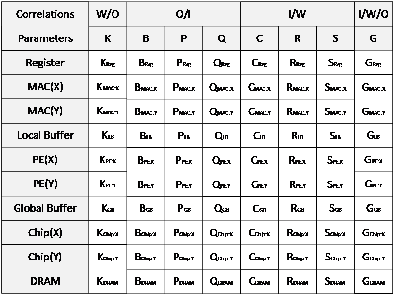
Figure 3: Scheduling Table Representation.

3.1.2.Scheduling Table Constraints

According to the definition of the scheduling table representation, the mapping values in the table must satisfy both the DNN parameter constraints and the hardware resource constraints. For the parameter constraints, the product of the values in each column of the scheduling table must equal the corresponding DNN parameter value. This ensures that the mapping respects the computational requirements of the neural network layers.

On the other hand, the hardware constraints require that the scheduling scheme take into account the actual hardware resources of the accelerator, ensuring that the storage capacity and computational capabilities of each component do not exceed their hardware limits [8]. For example, at the storage level, the size of the input, weight, and output data tiles must not exceed the cache capacity at that level, with data tile size calculated using the formulas provided in Table 2,\( i \)from a buffer level upwards to register. Similarly, for the spatial level, which pertains to the computational units, the product of the values in the corresponding row represents the number of hardware components involved in the computation at that level. This product must not exceed the total number of components available. The scheduling table must be optimized under these hardware constraints to maximize resource utilization and reduce conflicts.

Table 2: Formulas for calculating data tile sizes at each hardware level under resource constraints.

3.2.Reinforcement Learning Framework

Previous research has proposed both top-down and bottom-up optimization methods, however, both approaches are heuristic-based. A reasonable optimization method should not strictly adhere to either top-down or bottom-up approaches but should dynamically select the optimal scheduling sequence based on the scheduling context. Therefore, we transform the scheduling table’s mapping value optimization problem into an MDP, enabling the agent to select the optimal scheduling sequence based on the current scheduling state. The reinforcement learning agent iteratively optimizes the scheduling table by exploring different search orders and performing local optimizations, continuously improving its performance through iterative training.

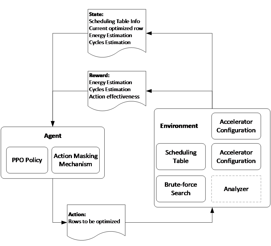
Figure 4: Reinforcement Learning Framework.

The reinforcement learning framework, illustrated in Figure 4, includes two main modules: the agent and the environment. The agent is the core of the reinforcement learning system. Its task is to obtain state information from the environment and select the optimal action based on the current scheduling state, following the current policy. The agent’s policy is continuously updated through interaction with the environment. In our implementation, we use Proximal Policy Optimization (PPO) to optimize the agent’s policy.

The environment defines the hardware configuration of the DNN accelerator, the parameters of the DNN layers, and the current mapping values and constraints in the scheduling table. During each iteration, the environment updates the current scheduling optimization state based on the actions selected by the agent and provides corresponding feedback. The feedback from the environment includes evaluations of the current scheduling state’s energy consumption, execution cycles, and the effectiveness of the action selected (e.g., whether there were redundant optimizations or multiple large-scale optimizations that failed to achieve better results). This feedback is used by the agent to update its policy, enabling better decisions in future scheduling actions.

The framework also defines the state space, action space, reward function, and the policy. The state space in reinforcement learning is a vector that describes the current system condition. In scheduling optimization, the state vector typically includes the current state of the scheduling table (i.e., the current mapping values, the components involved in the optimization, and the parameters of DNN layer), the available component for the next optimization step (represent as current optimized row\( r \)), the energy consumption and execution cycles of the current scheduling table. We use\( {s_{t}} \)to represent the state at step\( t \). The design of the state vector comprehensively reflects the current system status, enabling the agent to make optimal decisions based on this information.

The action space defines all possible actions the agent can take. In our design, an action refers to selecting which rows of the scheduling table to optimize. The agent can choose to optimize two or three rows in a single step, which are represented as\( [i, r] \)(\( i≠r \)and\( i∈[0, 9] \)) and\( [i, j, r] \)(\( i≠j≠r \)and\( i,j∈[0, 9] \)) respectively. The actions are encoded as\( {a_{t}}∈\lbrace k | k∈[0, 54]\rbrace \)to represent the action at step\( t \). If\( {a_{t}} \lt 10 \), the selected action is going to optimize two rows, otherwise, it is a multi-rows action.

The reward function measures whether the agent’s actions contribute to achieving the optimization goals. In our method, the reward function is defined based on energy consumption, execution cycles, and the effectiveness of the action taken. The reward function is shown in equation (1),\( {∆_{t}} \)is the difference between the optimized result and original result under the metric\( M \), and\( n \)is the number of consecutive multi-rows actions. If a scheduling strategy significantly reduces computation time or energy consumption, it will return a high reward. If the agent repeatedly chooses large-scale optimizations without yielding better results, it will receive a penalty. By optimizing the reward function, the agent can gradually learn the optimal scheduling strategy.

(1)

To effectively optimize the scheduling strategy within the reinforcement learning framework, we employ the PPO method. PPO defines a trust region to prevent drastic policy updates. Specifically, PPO uses a trust boundary to control the divergence between the new and old policies, ensuring that each update does not deviate too far from the current optimal policy [13]. The actor loss is using a clipped surrogate objective, which is shown in equation (2). The\( {π_{θ}} \)is the policy parameterized by\( θ \), and\( {A_{t}} \)is the advantage function computed using Generalized Advantage Estimation (GAE).

(2)

The critic loss is shown in equation (3), which integrates the L2 norm penalty with the Smooth L1 loss (Huber loss) to prevent overfitting while ensuring stable training. The\( {V_{ω}}(s) \)is the predicted state value at state\( s \), and\( {V_{ω}}(s \prime ) \)is the predicted state value at next state.

(3)

In our policy update method, we introduced entropy regularization (equation (4)) to the total loss, which encourages exploration by preventing the policy from becoming overly deterministic, thereby improving long-term performance. The total loss is shown in equation (5). The parameters\( {c_{1}} \)and\( {c_{2}} \)are the coefficients of value function and entropy, respectively, with\( {c_{2}} \)decaying over time to gradually reduce exploration as training progresses. The decaying function is shown in equation (6), its decay factor\( {λ_{{c_{2}}}} \)is set to\( 0.995 \). This approach ensures policy improvement while avoiding instability caused by excessive updates.

(4)

(5)

(6)

3.3.Action Masking

In the action space of reinforcement learning, certain actions may be invalid in specific states. For example, under certain hardware accelerator resource configurations, some rows in the scheduling table may correspond to hardware components that do not exist in the given accelerator, meaning that their mapping values should not participate in scheduling optimization. To improve the efficiency of the reinforcement learning algorithm, we introduce an action masking mechanism.

The basic principle of action masking is to filter out invalid actions in each state, thereby reducing the effective action space for the agent and improving training efficiency. In the implementation, action masking is performed by applying a binary mask to each action. When an action is invalid in the current state, the mask value is set to 0, indicating that the action is masked; when the action is valid, the mask value is set to 1, indicating that the agent can choose that action. Through this mechanism, the agent can more efficiently explore valid scheduling strategies, thus accelerating the learning process.

3.4.Brute-force Search for Locally Optimal Solutions

The reinforcement learning framework presented in this paper is designed to find an optimal scheduling sequence in a diverse scheduling optimization problem space and use a search method to identify the best scheduling strategy. This paper employs a brute-force search method, conducting an exhaustive search for locally optimal solutions within the specific rows selected for optimization during each action.

In scheduling optimization problem, the brute-force search first preprocesses the selected rows in the scheduling table to ensure the optimization satisfies the parameter constraints of the DNN layer. The detailed steps of the method are as follows:

•Preprocessing Step: First, the rows of the scheduling table selected by the action are preprocessed. The purpose of preprocessing is to multiply the mapping values in each column of the selected rows to obtain the parameter constraints corresponding to each parameter in those rows. For example, as shown in Fig. 5, after preprocessing, the products of the columns in each row are 2, 1, 14, and 7, respectively.

•Factorization and Exhaustive Search of Combinations: Once the products of the columns are obtained, this paper performs factorization to ensure that all possible scheduling combinations meet the parameter constraints. For instance, if the parameter value for P is 14, as shown in Figure 5. It needs to factorize it into values that can be used as mapping values for the hardware resources of the selected levels in the scheduling table. Through factorization, we can generate various potential mapping value combinations that satisfy the DNN layer's parameter constraints, such as {[1, 1, 14], [1, 14, 1], ..., [7, 2, 1]}. After completing factorization, we perform an exhaustive search of all possible scheduling combinations. For each possible combination, we map it into the scheduling table to form a complete scheduling plan.

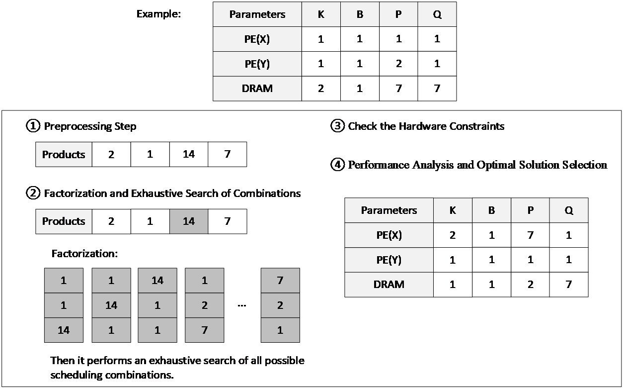
Figure 5: Example of Brute-force Search Method.

•Check the Hardware Constraints: During the exhaustive search process, some scheduling combinations may exceed the hardware resource limits of the accelerator, such as surpassing the capacity of local buffers or the number of processing elements. In these cases, the combinations that do not meet the hardware constraints are discarded. The remaining scheduling combinations are the valid ones that satisfy both hardware and parameter constraints.

•Performance Analysis and Optimal Solution Selection: For each valid scheduling combination, this paper perform an analysis of energy consumption and execution time. Based on the current optimization goal (e.g., minimizing energy consumption or execution time), we select the scheduling combination with the best performance as the locally optimal solution, thereby generating a more efficient scheduling table. As shown in Fig. 5, we select the optimal combination.

4.Experiment and Results Analysis

In this chapter, we validate the proposed reinforcement learning-based dataflow scheduling optimization method for DNN accelerators through a series of experiments. We first introduce the experimental setup, including the network structures and accelerator hardware configurations, as well as the tuning of hyperparameters. Then, we present the results of the experiments, demonstrating the effectiveness of the method in scheduling optimization, and compare it with other existing algorithms in terms of energy consumption and execution cycles.

4.1.Experimental Setup

For the experiments, we set the actor learning rate to\( 3×{10^{-4}} \), the critic learning rate to\( 1×{10^{-3}} \), the discount factor\( γ \)to\( 0.99 \), the clipping parameter\( ε \)to\( 0.2 \), the parameter of the L2 norm penalty\( {λ_{L2}} \)to\( 0.01 \), the coefficient of value function\( {c_{1}} \)to 0.5, the initial coefficient of entropy\( c_{2}^{0} \)to 0.1, and the final coefficient of entropy\( c_{2}^{final} \)to 0.02. Training was conducted up to 3000 episodes.

4.1.1.Deep Neural Network Configuration

To validate our proposed scheduling optimization method, we selected several representative deep neural network architectures for experiments, as shown in Table 3. These include YOLO v3, Inception v4, MobileNet v3, and ResNet-50 [15-17]. These networks have varying parameter configurations and computational requirements, providing a comprehensive evaluation of our method's generalization ability across different network architectures.

Table 3: DNN Models.

4.1.2.Accelerator Configuration

In terms of hardware configuration, we evaluated our method on multiple typical DNN accelerator architectures, as shown in Table 4, including Eyeriss, TPU, and Simba [18-21]. These accelerators feature varying hardware resource configurations, allowing us to assess the effectiveness of our model across different hardware setups.

Table 4: Accelerator Architecture Component Configurations.

4.2.Accuracy Analysis of Scheduling Optimization

To further verify the superiority of our proposed method, we compared it with other existing scheduling optimization algorithms. Specifically, we selected the commonly used DNN accelerator scheduling methods, such as Timeloop, CoSA, ZigZag, and NeuroSpector, as baselines and conducted experiments using the same network architectures and hardware configurations [8,9,11,12].

4.2.1.Energy Consumption Comparison

In the energy efficiency comparison experiments, we measured the energy consumption of each algorithm across different network architectures and accelerator configurations. The Table 5 compares the energy consumption of NeuroSpector (N) and RL-Scheduling (RL). It shows that RL-Scheduling consistently improves energy efficiency across most models with different accelerators. For YOLO v3, RL-Scheduling reduces energy consumption by about 7.3% on Eyeriss and 1.8% on TPU v3 compared to NeuroSpector. In MobileNet v3, it provides around 4.6% and 5.2% energy reduction on Eyeriss and Simba, respectively, while showing similar performance to NeuroSpector on TPU v3. For ResNet-50, RL-Scheduling achieves a 13.4% reduction on Eyeriss, with minimal differences on other accelerators.

Table 5: Energy Consumption Comparison of NeuroSpector (N) and RL-Scheduling (RL) Methods Across Different DNN Models and Accelerators.

The experimental results on Eyeriss comparing with other methods is shown in Figure 7. The methods include Timeloop (T), CoSA (C), ZigZag (Z), NeuroSpector (N), and RL-Scheduling (RL). For YOLO v3, RL-Scheduling reduces energy consumption by approximately 59.7% compared to Timeloop and by about 38.2% compared to CoSA. In Inception v4, RL-Scheduling shows a similar trend, with about a 52.7% reduction in energy consumption compared to Timeloop and a 47.8% reduction compared to CoSA. For MobileNet v3, where Timeloop and CoSA did not provide results, RL-Scheduling achieves similar performance to NeuroSpector and ZigZag.

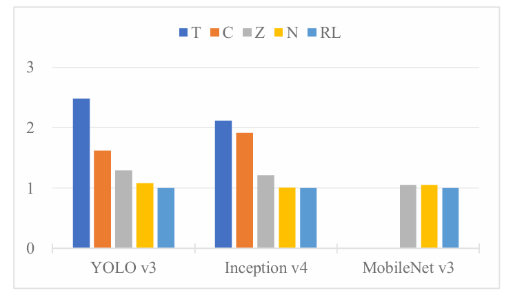
Figure 7: Energy Consumption Comparison of Scheduling Methods on Eyeriss for YOLO v3, Inception v4, and MobileNet v3.

4.2.2.Execution Cycle Comparison

In terms of execution cycles, our method also demonstrated significant advantages. The Table 6 compares the execution cycles after the scheduling optimization by NeuroSpector (N) and RL-Scheduling (RL). For YOLO v3, RL-Scheduling reduces the number of cycles by about 26.7% on Eyeriss and 1.3% on TPU v3 compared to NeuroSpector. In Inception v4, RL-Scheduling achieves a 4.1% cycle reduction on Eyeriss. In MobileNet v3, it provides around 10.1% cycle reduction on Eyeriss, while showing similar performance to NeuroSpector on TPU v3. For ResNet-50, RL-Scheduling achieves a 31.5% reduction on Eyeriss, with minimal differences on other accelerators.

Table 6: Execution Cycle Comparison of NeuroSpector (N) and RL-Scheduling (RL) Methods Across Different DNN Models and Accelerators.

The experimental results on TPU v3, as shown in Figure 8, demonstrate significant improvement with RL-Scheduling. For YOLO v3, RL-Scheduling reduces execution cycles by approximately 65.6% compared to Timeloop, while CoSA, and ZigZag failed to produce results. In Inception v4, RL-Scheduling achieves a 61.5% reduction in cycles compared to Timeloop, while CoSA, and ZigZag again unabled to provide results. For MobileNet v3, RL-Scheduling performs similarly to NeuroSpector, while Timeloop, CoSA, and ZigZag failed to produce results.

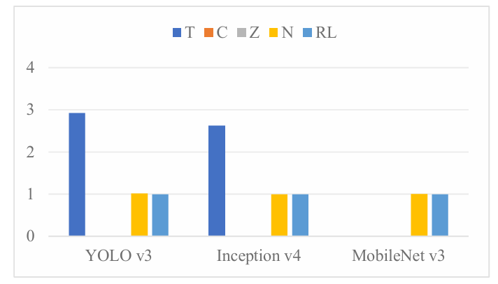
Figure 8: Execution Cycle Comparison of Scheduling Methods on TPU v3 for YOLO v3, Inception v4, and MobileNet v3.

4.3.Comparison of Algorithm Efficiency

In this experiment, we compared the runtime of different scheduling methods on Eyeriss for YOLO v3, Inception v4, and MobileNet v3, as shown in Figure 9. The methods evaluated include Timeloop (T), CoSA (C), ZigZag (Z), NeuroSpector (N), and RL-Scheduling (RL).

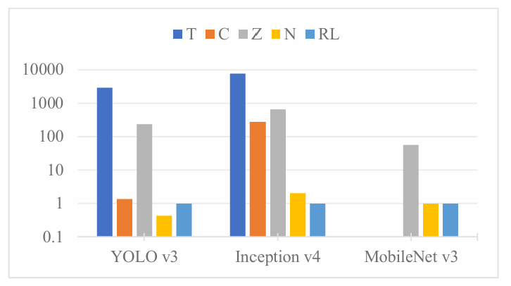
Figure 9: Runtime Comparison of Scheduling Methods on Eyeriss for YOLO v3, Inception v4, and MobileNet v3.

In YOLO v3, RL-Scheduling reduces runtime by over 99% compared to Timeloop (T) and ZigZag (Z), while performing similarly to CoSA (C) but slightly worse than NeuroSpector (N). In Inception v4, RL-Scheduling achieves a runtime reduction of over 99% compared to T, C, and Z, and a 51.5% reduction compared to N. In MobileNet v3, RL-Scheduling reduces runtime by nearly 99% compared to Z and performs on par with N, while T and C failed to provide results.

4.4.Experimental Summary

The results of the above experiments validate the effectiveness and superiority of the reinforcement learning-based scheduling optimization method for DNN accelerators. The experimental results show that the proposed method not only reduces energy consumption and improves overall computational efficiency, but also enables targeted optimization for different types of DNN layers. Additionally, compared to existing scheduling algorithms, the reinforcement learning method is better able to explore the optimal solutions in large design spaces, demonstrating stronger generalization and stability.

5.Conclusion

In this paper, we presented a reinforcement learning-based framework for optimizing dataflow scheduling in DNN accelerators. By employing Proximal Policy Optimization (PPO) alongside a brute-force search for locally optimal solutions, our approach adapts dynamically to hardware resource constraints and DNN workload requirements. The experimental results showed significant improvements in both energy consumption and execution cycles compared to traditional scheduling methods. The framework demonstrates scalability across different DNN models and hardware configurations, offering a robust solution for accelerating deep learning tasks with optimized performance.

As the complexity of DNN models continues to grow, the design of accelerator architectures has become increasingly intricate, placing greater demands on the generalization capability of scheduling models. Although the PPO-based reinforcement learning framework has demonstrated effectiveness in scheduling optimization, its efficiency decreases in large state spaces, leading to slower convergence and reduced search effectiveness, which limits its application in complex DNN tasks. Future research should focus on refining the definition of the state space by incorporating encoder techniques to enhance search efficiency, and on improving the generalization capabilities of the model, ensuring consistent performance across diverse DNN architectures and hardware accelerators. These advancements will help make reinforcement learning-based scheduling methods more scalable and adaptable.

References

[1]. Jouppi N P, Young C, Patil N, et al. In-datacenter performance analysis of a tensor processing unit. Proceedings of the 44th annual international symposium on computer architecture. 2017: 1-12.
[2]. Liu D, Yin S, Luo G, et al. Data-flow graph mapping optimization for CGRA with deep reinforcement learning. IEEE Transactions on Computer-Aided Design of Integrated Circuits and Systems, 2018, 38(12): 2271-2283.
[3]. Blanco F G, Russo E, Palesi M, et al. Deep Reinforcement Learning based Online Scheduling Policy for Deep Neural Network Multi-Tenant Multi-Accelerator Systems. arXiv preprint arXiv:2404.08950, 2024.
[4]. AMohaidat T, Khalil K. A survey on neural network hardware accelerators. IEEE Transactions on Artificial Intelligence, 2024.
[5]. Latotzke C, Gemmeke T. Efficiency versus accuracy: a review of design techniques for DNN hardware accelerators. IEEE Access, 2021, 9: 9785-9799.
[6]. Bause O, Bernardo P P, Bringmann O. A Configurable and Efficient Memory Hierarchy for Neural Network Hardware Accelerator. arXiv preprint arXiv:2404.15823, 2024.
[7]. Wang C, Wang Z, Li S, et al. EWS: An Energy-Efficient CNN Accelerator With Enhanced Weight Stationary Dataflow. IEEE Transactions on Circuits and Systems II: Express Briefs, 2024.
[8]. Parashar A, Raina P, Shao Y S, et al. Timeloop: A systematic approach to dnn accelerator evaluation. 2019 IEEE international symposium on performance analysis of systems and software (ISPASS). IEEE, 2019: 304-315.
[9]. Huang Q, Kang M, Dinh G, et al. Cosa: Scheduling by constrained optimization for spatial accelerators. 2021 ACM/IEEE 48th Annual International Symposium on Computer Architecture (ISCA). IEEE, 2021: 554-566.
[10]. Hegde K, Tsai P A, Huang S, et al. Mind mappings: enabling efficient algorithm-accelerator mapping space search. Proceedings of the 26th ACM International Conference on Architectural Support for Programming Languages and Operating Systems. 2021: 943-958.
[11]. Mei L, Houshmand P, Jain V, et al. ZigZag: Enlarging joint architecture-mapping design space exploration for DNN accelerators. IEEE Transactions on Computers, 2021, 70(8): 1160-1174.
[12]. Park C, Kim B, Ryu S, et al. NeuroSpector: Systematic Optimization of Dataflow Scheduling in DNN Accelerators. IEEE Transactions on Parallel and Distributed Systems, 2023, 34(8): 2279-2294.
[13]. Ma D. Reinforcement learning and autonomous driving: Comparison between DQN and PPO. AIP Conference Proceedings. AIP Publishing, 2024, 3144(1).
[14]. Adarsh P, Rathi P, Kumar M. YOLO v3-Tiny: Object Detection and Recognition using one stage improved model. 2020 6th international conference on advanced computing and communication systems (ICACCS). IEEE, 2020: 687-694.
[15]. Szegedy C, Ioffe S, Vanhoucke V, et al. Inception-v4, inception-resnet and the impact of residual connections on learning. Proceedings of the AAAI conference on artificial intelligence. 2017, 31(1).
[16]. Howard A, Sandler M, Chu G, et al. Searching for mobilenetv3. Proceedings of the IEEE/CVF international conference on computer vision. 2019: 1314-1324.
[17]. Koonce B, Koonce B. ResNet 50. Convolutional neural networks with swift for tensorflow: image recognition and dataset categorization, 2021: 63-72.
[18]. Chen Y H, Krishna T, Emer J S, et al. Eyeriss: An energy-efficient reconfigurable accelerator for deep convolutional neural networks. IEEE journal of solid-state circuits, 2016, 52(1): 127-138.
[19]. Chen Y H, Yang T J, Emer J, et al. Eyeriss v2: A flexible accelerator for emerging deep neural networks on mobile devices. IEEE Journal on Emerging and Selected Topics in Circuits and Systems, 2019, 9(2): 292-308.
[20]. Norrie T, Patil N, Yoon D H, et al. The design process for Google's training chips: TPUv2 and TPUv3. IEEE Micro, 2021, 41(2): 56-63.
[21]. Shao Y S, Clemons J, Venkatesan R, et al. Simba: Scaling deep-learning inference with multi-chip-module-based architecture. Proceedings of the 52nd Annual IEEE/ACM International Symposium on Microarchitecture. 2019: 14-27.
Cite this article
Xu,F. (2025). Reinforcement Learning-Based Scheduling Optimization for DNN Accelerators. Applied and Computational Engineering,123,177-191.
Data availability
The datasets used and/or analyzed during the current study will be available from the authors upon reasonable request.
Disclaimer/Publisher's Note
The statements, opinions and data contained in all publications are solely those of the individual author(s) and contributor(s) and not of EWA Publishing and/or the editor(s). EWA Publishing and/or the editor(s) disclaim responsibility for any injury to people or property resulting from any ideas, methods, instructions or products referred to in the content.
About volume
Volume title: Proceedings of the 5th International Conference on Materials Chemistry and Environmental Engineering
© 2024 by the author(s). Licensee EWA Publishing, Oxford, UK. This article is an open access article distributed under the terms and
conditions of the Creative Commons Attribution (CC BY) license. Authors who
publish this series agree to the following terms:
1. Authors retain copyright and grant the series right of first publication with the work simultaneously licensed under a Creative Commons
Attribution License that allows others to share the work with an acknowledgment of the work's authorship and initial publication in this
series.
2. Authors are able to enter into separate, additional contractual arrangements for the non-exclusive distribution of the series's published
version of the work (e.g., post it to an institutional repository or publish it in a book), with an acknowledgment of its initial
publication in this series.
3. Authors are permitted and encouraged to post their work online (e.g., in institutional repositories or on their website) prior to and
during the submission process, as it can lead to productive exchanges, as well as earlier and greater citation of published work (See
Open access policy for details).