1. Introduction

The quest for sustainable and clean energy sources has become one of the most pressing challenges of our time, as the world grapples with the dual crises of climate change and dwindling fossil fuel reserves. Solar energy, with its vast potential and minimal environmental footprint, stands at the forefront of this quest. My journey into the solar energy sector began with an internship at Jinko Solar’s China division, where I was immersed in the rapidly evolving world of energy development. This invaluable experience, coupled with my participation in the design of two solar power station projects, not only broadened my understanding of solar photovoltaic (PV) technology but also deepened my appreciation for clean energy’s pivotal role in preserving our planet’s future.

One challenge in the field of solar energy is to improve the efficiency of bifacial solar panels, which absorb not only sunlight from the front but also light reflected in the environment from the back, thereby significantly increasing energy output. However, despite their potential, the widespread adoption of bifacial solar panels has been hampered by cost and efficiency barriers.

Based on my experience and the urgent need for efficient renewable energy solutions, this project aims to dramatically increase the productivity of bifacial solar panels. By integrating dynamic sun tracking and mirror array systems, I aim to increase the energy efficiency of standard bifacial solar panels by 140%. Specifically, the optimized PV system aims to achieve annual power generation of 130 kWh per square meter in Tucson, Arizona, which has one of the highest solar irradiance levels in the United States. This ambitious target not only meets the demand for higher energy production from solar installations, but also aligns with the global Sustainable Development Goals.

The core of this CRD is the detailed design of the system, which includes the selection of critical components, the creation of CAD models, the establishment of computational methods for system optimization, an analysis of potential errors, code for an algorithm, simulation in Lighttools and analysis of simulation results.

2. System Architecture

2.1. System block diagram

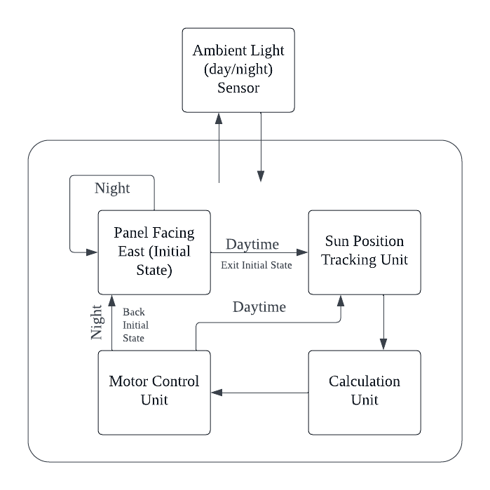
Figure 1: System block diagram

2.2. System Block Diagram Description

In the pre-dawn state, the solar panels are positioned due east, primed for initial sun capture. The system's 'Ambient Light (day/night) Sensor' discerns the ambient light level, serving as the diurnal transition trigger. Upon sunrise detection, a signal is dispatched to the 'Sun Position Tracking Unit,' a component that tuns with the solar panel to pinpoint the 3D angle (X-axis angle and Y-axis angle) of the sun relative to the system.

At the same time, the "computing unit" processes the position data of the sun to determine how best to reflect sunlight onto the back surface of the two-sided panel and adjusts the stepper motors behind each mirror to adjust their angles, maximizing energy capture by utilizing both direct and reflected light.

Throughout the day, this process is meticulously repeated at 30-minute intervals, guaranteeing constant alignment with the sun's trajectory. When daylight wanes and the ambient light sensor records that there is not enough sunlight, a dusk signal is issued, and the system commands all panels and mirrors to reset to their initial positions. Each motor ensures that the solar panels face east, ready to restart the cycle at the next sunrise, while the mirrors are set to a neutral position to avoid unnecessary exposure and potential nighttime damage.

3. Ana Analysis and preparation before simulation

3.1. Sun simulation

The sun, acting as the light source in simulation experiments, necessitates accurate representation of its movement throughout the day. Since it is difficult to find data on solar radiation per hour for cities in the United States, I decided to use the solar constant for the simulations within LightTools. A simplified way to estimate the diurnal variation in solar radiation intensity is to consider the Angle between a point on the Earth's surface and the sun's rays, known as the solar altitude Angle. When the sun is above the horizon, the solar altitude Angle is higher, and the path of solar radiation through the atmosphere is shorter, scattering and absorption are less, so more solar energy is received. Conversely, when the sun is near the horizon (such as at sunrise and sunset), the sun's light takes a longer path through the atmosphere, scattering and absorbing more, and therefore receiving less energy. The carination of solar radiation over the course of a day can be roughly described by the cosine law: , where I is the intensity of solar radiation received by the ground, is the solar constant, is the Angle of the sun’s rays perpendicular to the ground, the remaining Angle of the sun’s altitude Angle. At the same time, we will set the ground to a diffuse reflection with a reflectivity of 0.1 to simulate the land. This streamlined approach facilitates a realistic simulation of diurnal solar radiation changes without complex data.

Under these conditions, LightTools simulates the daily output of bifacial solar panels with and without a mirror array and sun tracking system to calculate a rough ratio, which is then taken into Tucson’s annual irradiance to calculate its annual power output.

3.2. Sun tracking

The sun tracking system described utilizes a pair of orthogonally arranged solar sensors, each consisting of a narrow aperture leading to a photodiode at its base. This system is engineered to dynamically orient itself towards the sun through the precise operation of stepper motors. When sunlight streams directly down the slit and impinges on the photodiode, the system’s control computer registers this alignment, marking the precise solar angle in one dimension. Subsequently, the system adjusts in the perpendicular plane, seeking a similar direct illumination on the second sensor. Achieving direct sunlight on both sensors allows the computer to computer to compute the sun’s 3D position relative to the sun tracker.

The inherent width of the slits, though minimized, cannot be reduced to an ideal zero, thus conferring a finite field of view angle to each sensor. This characteristic introduces a marginal degree of error in the system’s solar tracking accuracy. The distance between the top of slit to the sensor is 116.9 mm, and the distance from the edge of one side of the sensor’s active area of the sensor to the wall on the other side of the slit is 4.55 mm. The error is:

\( Error=HFOV={cos^{-1}}{(\frac{116.9 mm}{4.55 mm})=1.5708°} \)

In theoretical terms, the system’s capacity of sun angle alignment is within \( ± 1.5708° \) . This fully meets the expected design sun-tracking error of \( ± 5° \) . However, in practical applications, considerations such as manufacturing tolerances, thermal expansion, and component wear can lead to variations in this precision.

3.3. Calculation

Upon receiving the solar azimuth and elevation angles from the sun tracking system, the system initiates a computation to ascertain the optimal reflection angles for each mirror. The methodology underlying this angle calculation, which is essential for maximizing the photovoltaic efficiency of the system. This figure outlines the mathematical derivation that informs the precise positioning of the mirrors to ensure the bifacial solar panels are exposed to the maximum possible sunlight.

Point A is the position of sun tracker, point S is the position of sun, and \( {θ_{s}} \) is the relative Angle between sun and sun tracker in one-axis. Point B is the position of irradiation target, point M is the position of mirror, and point E is the projection of point M onto the X-axis. The projection of the Sun's position on the X-axis is point C, and the line between the sun and the mirror intersects the X-axis at point D. When we install the entire solar system, we record in the computer the position of each component and the distance between them.

The target is to calculate the tilt angle \( {θ_{t}} \) . Set the distance between sun tracker and sun AS is approximately to \( 150*{10^{9}} m \) . Because the distance AB, BE, AE, EM are fixed, so the angle

\( ∠EBM=atan{(\frac{BE}{EM})}\ \ \ (1) \)

is fixed. With the \( {θ_{s}} \) , that received from sun tracker, we can get the

\( AC=AS*sin{({θ_{s}})}\ \ \ (2) \)

\( CS=A*cos{({θ_{s}})}\ \ \ (3) \)

Then

\( CE=AE-AC=AE-AS*sin({θ_{s}})\ \ \ (4) \)

Set \( CD=x \) , \( DE=CE-x \) , and because

\( ∠DSC=∠DME=θ_{s}^{ \prime }\ \ \ (5) \)

\( \frac{x}{CS}=\frac{CE-x}{EM}=tan{(θ_{s}^{ \prime })}\ \ \ (6) \)

Therefor,

\( x=\frac{CE*CS}{EM+CS}\ \ \ (7) \)

Then, we got:

\( θ_{s}^{ \prime }={tan^{-1}}{(\frac{CE}{EM+CS})}={tan^{-1}}{(\frac{AE-AS*sin{({θ_{s}})}}{EM+AS*cos{({θ_{s}})}})}\ \ \ (8) \)

\( 2{θ_{M}}=∠DMB=∠EMB-θ_{s}^{ \prime }\ \ \ (9) \)

\( {θ_{t}}=90°-∠EBM-{θ_{M}}=90°-{tan^{-1}}{(\frac{BE}{EM})}-\frac{1}{2}({tan^{-1}}{(\frac{BE}{EM})}-{tan^{-1}}{(\frac{AE-AS*sin{({θ_{s}})}}{EM+AS*cos{({θ_{s}})}})})\ \ \ (10) \)

\( {θ_{t}}=90°-\frac{3}{2}{tan^{-1}}{(\frac{BE}{EM})}+{tan^{-1}}{(\frac{AE-AS*sin{({θ_{s}})}}{EM+AS*cos{({θ_{s}})}})}\ \ \ (11) \)

With the acquisition of 2 \( {θ_{s}} \) values representing the sun’s position, we can delineate the angles \( {θ_{tx}} \) and \( {θ_{ty}} \) within the X-Z and X-Y planes, respectively. These angles are then transformed into spherical coordinates as \( θ \) and \( ϕ \) .

In this context, since the problem’s focus excludes considerations of length, maintaining the ratios of the trigonometric functions suffices. By setting \( z=1 \) , we define \( x=sin{({θ_{tx}})} \) and \( y=sin{({θ_{ty}})} \) , then,

\( θ=arctan{(\frac{\sqrt[]{{x^{2}}+{y^{2}}}}{z})}=arctan(\frac{\sqrt[]{{sin^{2}}{({θ_{tx}})}+{sin^{2}}{({θ_{ty}})}}}{1})=arctan{(\sqrt[]{{sin^{2}}{({θ_{tx}})}+{sin^{2}}{({θ_{ty}})}})}\ \ \ (12) \)

\( ϕ=arctan{(\frac{y}{x})}=arctan{(\frac{sin{({θ_{ty}})}}{sin{({θ_{tx}})}})}\ \ \ (13) \)

3.4. Motor control

In calculating θ and φ within these spherical coordinates, θ represents the motor's orientation angle that adjusts the azimuth, whereas φ denotes the orientation angle for the motor controlling the elevation. This distinction is crucial for the precise manipulation of the solar tracking system, ensuring that each motor is aligned according to the specific directional adjustments required for optimal solar irradiation capture.

4. Simulation

4.1. Set up in LightTools

This section encompasses three aspects: setting up the solar model, modeling the bifacial solar panel, and configuring the mirror array.

After discussing with the teaching assistant and classmates, I discovered the Solar Source Utility tool within LightTools. This utility allows me to set up a solar light source directly by specifying the location and time. Although it does not have an option for Tucson specifically, I chose Phoenix as the closest available location. This configuration enabled me to simulate a realistic solar model.

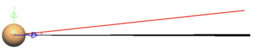
Figure 2: Sun simulation

The resulting solar model features a distant Lambertian light source that also simulates atmospheric scattering, closely resembling real-world solar illumination. With the solar model ready, I inserted a 1-meter-wide square plate to represent the bifacial solar panel. Both sides of the panel were configured as surface receivers to accurately capture sunlight from multiple angles.

Next, I created a mirror array consisting of four discs, each with a 50 cm radius. These mirrors are positioned 50 cm away from the solar panel center in the x, y, and z directions. The optical properties of the side facing the solar panel were set to mirror to reflect sunlight effectively.

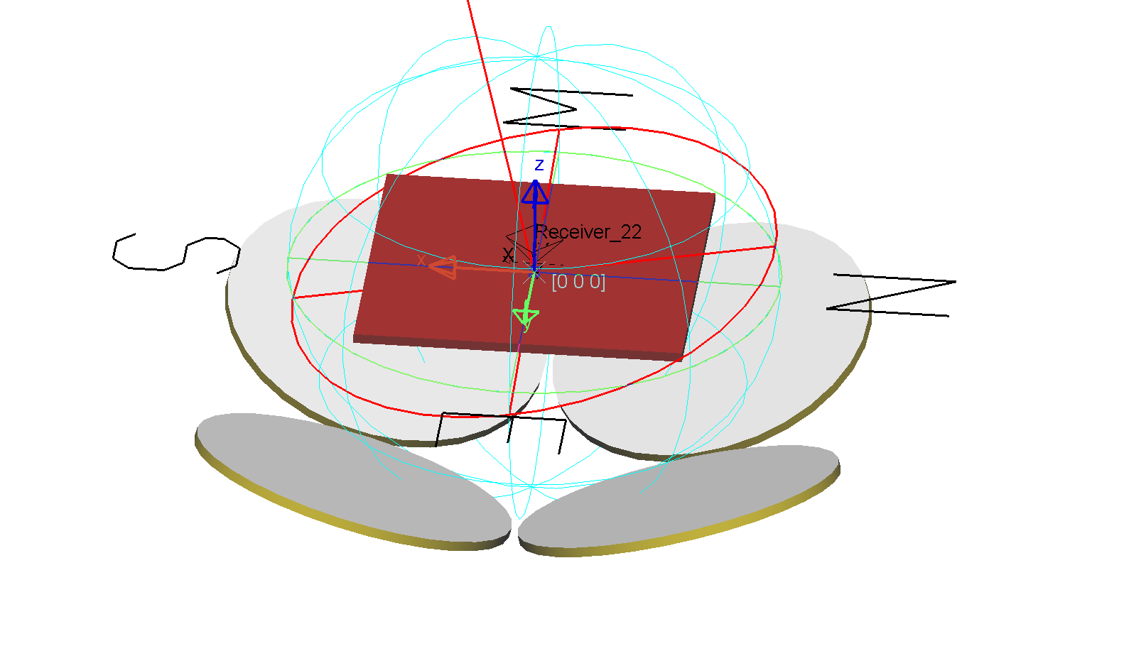
Figure 3: bifacial solar panel with mirror array condenser system

4.2. MATLAB code

The MATLAB code is tailored to calculate the alpha and beta angles for all four mirrors simultaneously. This ensures that each mirror is optimally oriented to reflect sunlight toward the bifacial solar panel, maximizing the overall energy capture. Although the Solar Source Utility in LightTools can generate a solar model for illumination, it does not directly provide specific solar angle data. Instead, the sun's azimuth and elevation angles are available through the NOAA ESRL Global Monitoring Laboratory website.

The Azimuth angle measures the sun's position relative to the horizon in a clockwise direction from true north. It helps in determining the horizontal direction of sunlight. And the elevation angle indicates the vertical position of the sun relative to the horizon, ranging from 0° (horizon) to 90° (overhead).

To accurately orient the mirrors, the azimuth and elevation angles of sun need to be converted into the alpha and beta angles required for computational purposes. After determining the correct conversion formulas, the results are implemented in the MATLAB code. Each of the four mirrors is positioned 50 centimeters from the solar panel in the x, y, and z directions. Thus, the only modification needed is to assign the appropriate sign for each direction to obtain the correct alpha and beta angles. This way, all four mirrors are oriented properly with a single calculation.

This approach provides an efficient way to ensure all mirrors reflect sunlight effectively, maximizing energy capture and ensuring the system operates at peak efficiency.

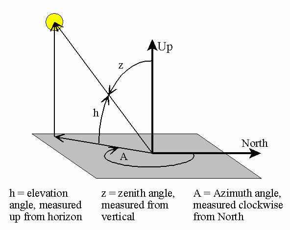
Figure 4: Azimuth/Elevation/Zenith Figure

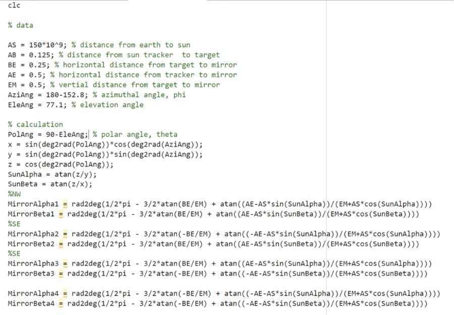
Figure 5: MATLAB code

4.3. Simulation

The simulation in this part is limited due to ongoing debugging of the MATLAB code, so only a simulation at noon (12:00 PM) has been conducted. This simulation uses the solar source, mirrors, and bifacial solar panel set up previously in Part 6.1.

Each mirror requires specific alpha and beta angles, which are obtained through calculations from the MATLAB code. Once these angles are calculated, they are manually input into the simulation model for each mirror, ensuring accurate positioning relative to the solar source.

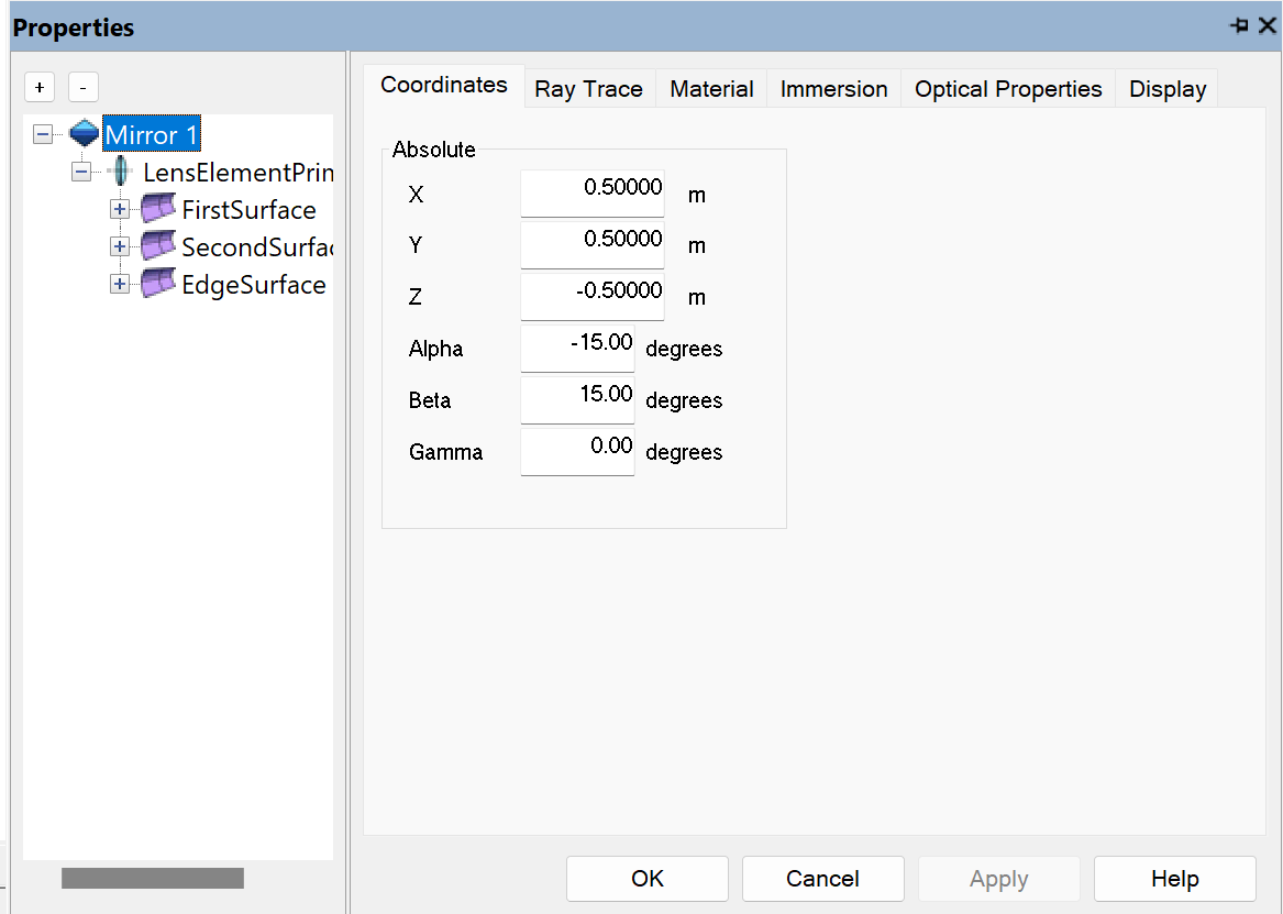
Figure 6: properties of mirror

With the solar source configured using the Solar Source Utility, and the mirror surfaces and bifacial panel already set up, the simulation proceeds by simply initiating the ray tracing functionality. The rays from the solar source are traced to the mirrors, where they are reflected onto the bifacial solar panel. This setup allows for real-world-like performance testing of the mirror array and panel, which helps refine the model for maximum efficiency.

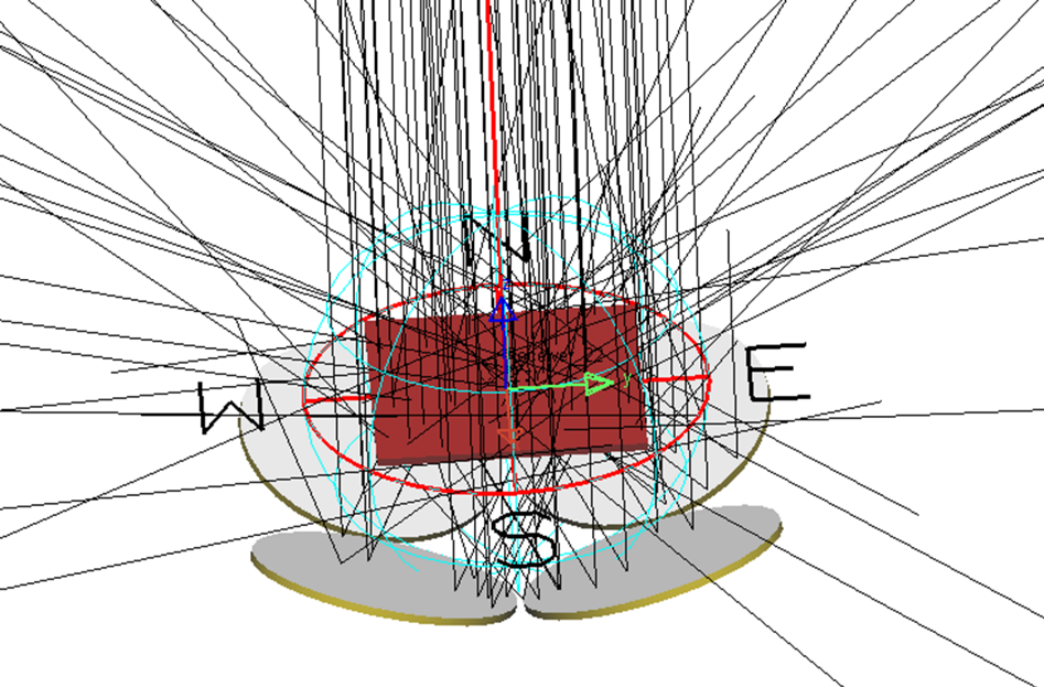
Figure 7: Ray tracing

4.4. Result and analysis

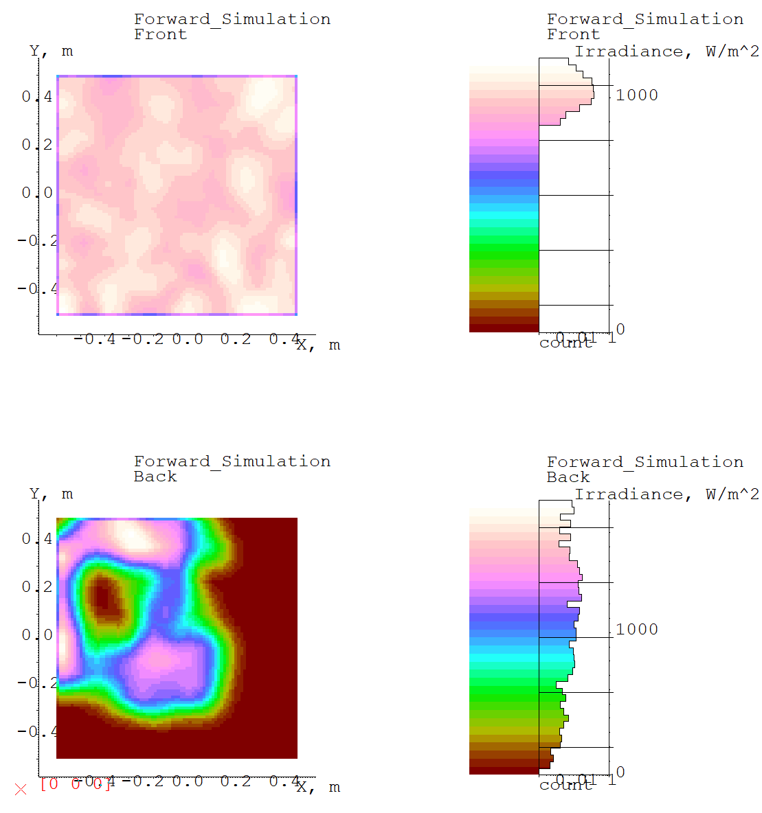
Figure 8: Chart illumination data of front and back of panel

From figure 8, we know the irradiation on the front surface of bifacial panel is 1031.6 W, and the irradiation on the back surface is 535.57. Which means the back surface increases the total power by

\( \frac{535.57 W}{1031.6 W}×100\%=51.916\% \)

Since we can only simulate 12 noon at the moment, let's consider the increase rate as the result of the whole day. Next, we can calculate the daily irradiation with Parameter Analyzer tool in Solar Source.

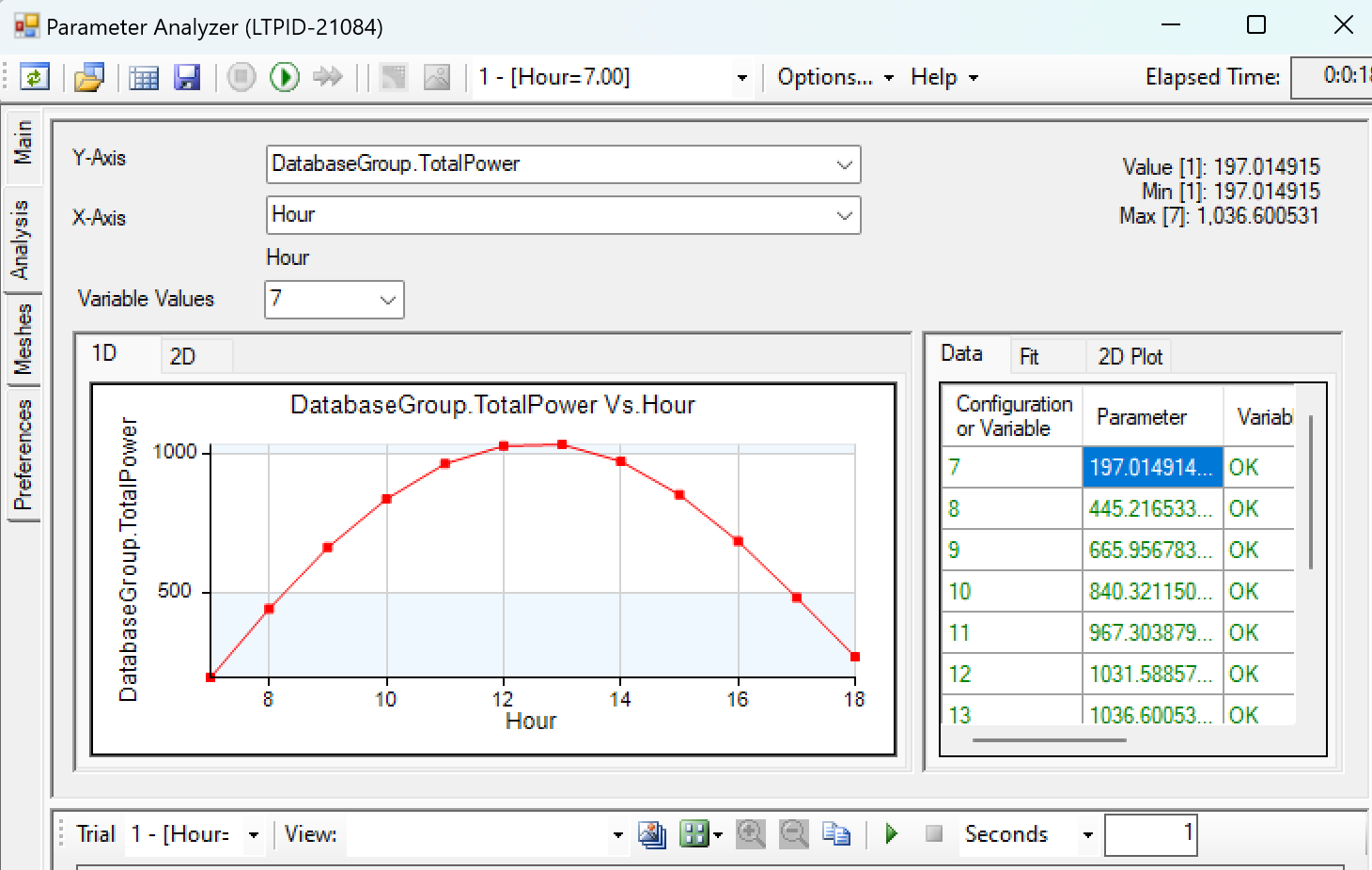
Figure 9: Daily irradiation.

With the data from Parameter Analyzer, the daily irradiation on May 30^th in Phoenix is approximately 8461.719 Wh/m². Then we simulate the power for the whole month.

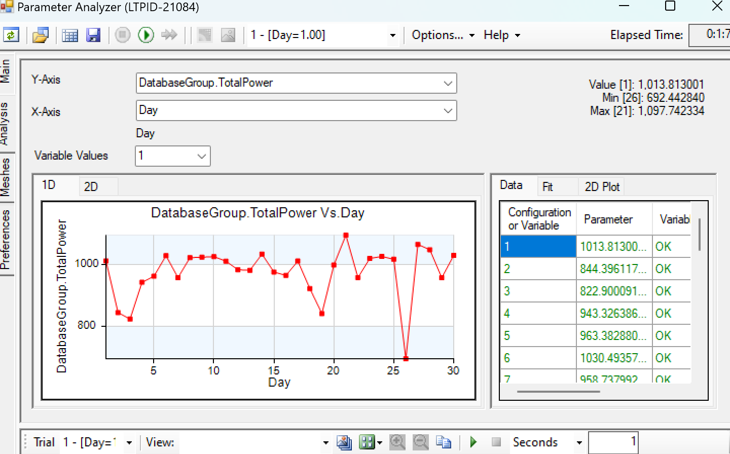
Figure 10: Monthly irradiation

With the irradiation data on May 30th, I can calculate the ratio and get the monthly irradiation of May is 240475.507 Wh/m2. Next, we simulate the irradiation for the whole year.

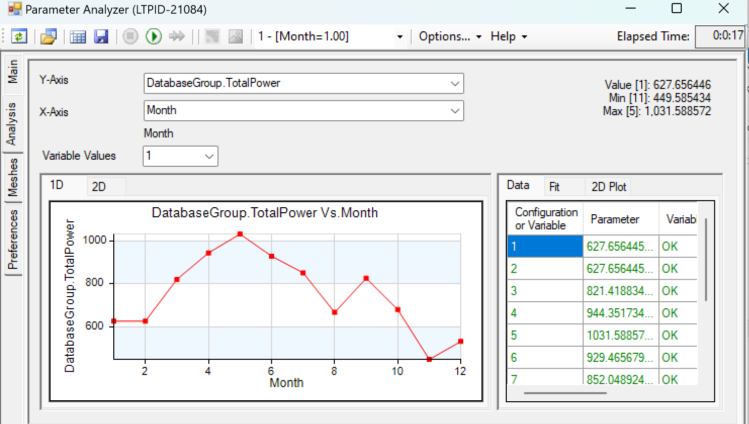
Figure 11: Annual irradiation

The annual irradiation is about 419211.901 Wh/m2, which is about 420 kWh/m2. The JKM560N-72HL4-BDV bifacial solar panel we selected has a module efficiency of 21.68%, with the 51.916% of incremental of our system, the annual electricity generation is

\( 420 kWh/{m^{2}}×21.68\%×(1+51.916\%)=138.329 kWh/{m^{2}} \)

The optimized PV system can achieve annual power generation of 138 kWh per square meter in Phoenix, Arizona, which means it meets the design requirement, 130 kWh/m2 in Tucson, Arizona. Because Tucson's latitude is smaller than Phoenix's, its annual solar irradiation will only be greater than Phoenix's, so the electricity generation must be greater.

5. Conclusion

In this Critical Design Review, we've thoroughly analyzed and validated the solar energy system's design, modeling, and simulation. This review demonstrated that our simulation environment, combining LightTools and MATLAB, successfully established a detailed solar source model using the Solar Source Utility. The bifacial solar panel and mirror array were both carefully designed to optimize energy capture. Despite challenges encountered during debugging, the MATLAB code proved effective in calculating mirror angles to reflect solar energy optimally toward the panel. And our optimized PV system can achieve annual power generation of 138 kWh per square meter in Phoenix, Arizona, which is exceeded our expectations.

The integration plan for LightTools and external control software presents an opportunity for dynamic, real-time mirror adjustments, promising continued optimal energy capture under varying solar conditions. This seamless interaction between software and hardware is crucial to maintaining efficiency.

During the process, we recognized the importance of iterative testing in simulation environments, especially in debugging the MATLAB code. The plan for dynamic mirror adjustments emphasized the challenges of processing and synchronizing real-time data across simulation and hardware systems. The implementation of this plan requires careful refinement and validation to ensure accurate data processing and smooth execution.

Moving forward, refining the MATLAB code remains a priority to guarantee reliable mirror angle calculations across all conditions. Implementing and rigorously testing real-time adjustments between LightTools and external control programs will be essential in validating their effectiveness. Further simulations will help uncover potential optimizations in mirror array design and positioning, ultimately leading to a highly efficient solar energy system.

References

[1]. Energy Information Agency (EIA). 2023. “How much of the U.S. carbon dioxide emissions are associated with electricity generation?”
[2]. Epstein, P.R.,J. J. Buonocore, K. Eckerle, M. Hendryx, B. M. Stout III, R. Heinberg, R. W. Clapp, B. May, N. L. Reinhart, M. M. Ahern, S. K. Doshi, and L. Glustrom. 2011. Full cost accounting for the life cycle of coal in “Ecological Economics Reviews.” Ann. N.Y. Acad. Sci. 1219: 73–98.
[3]. Deyette, J., and B. Freese. 2010. “Burning coal, burning cash: Ranking the states that import the most coal.” Cambridge, MA: Union of Concerned Scientists.
[4]. Koshel, R. John. Illumination Engineering. 1. Aufl. Newark: Wiley-IEEE Press, 2012. Print.
[5]. Jinko, JKM560-72HL4, JKM560-580N-72HL4-BDV-F4-EN.pdf (shwebspace.com)
[6]. Jose A. Carballo, Javier Bonilla, Lidia Roca, Manuel Berenguel, New low-cost solar tracking system based on open source hardware for educational purposes, Solar Energy, Volume 174, 2018, Pages 826-836,ISSN 0038-092X, https://doi.org/10.1016/j.solener.2018.09.064.
[7]. Thorlabs, FD11A, Thorlabs - FD11A Si Photodiode, 400 ns Rise Time, 320 - 1100 nm, 1.1 mm x 1.1 mm Active Area
[8]. PHOTOVOLTAIC GEOGRAPHICAL INFORMATION SYSTEM, JRC Photovoltaic Geographical Information System (PVGIS) - European Commission (europa.eu)
[9]. Kalikinkar Bandyopadhyay, Pramila Aggarwal, Debashis Chakraborty, Sanatan Pradhan, Practical Manual on Measurement of Soil Physical Properties Practical, March 2012
[10]. Solar Energy & Solar Power in Tucson, AZ | Solar Energy Local
[11]. Bernie Outram, Black Coatings to Reduce Stray Light, Black-Coatings-to-Reduce-Stray-Light.pdf (arizona.edu)
[12]. Solar Position Calculator, NOAA ESRL
Cite this article
Chen,W. (2025). Bifacial Solar Panel with Mirror Condenser System. Applied and Computational Engineering,124,165-174.
Data availability
The datasets used and/or analyzed during the current study will be available from the authors upon reasonable request.
Disclaimer/Publisher's Note
The statements, opinions and data contained in all publications are solely those of the individual author(s) and contributor(s) and not of EWA Publishing and/or the editor(s). EWA Publishing and/or the editor(s) disclaim responsibility for any injury to people or property resulting from any ideas, methods, instructions or products referred to in the content.
About volume
Volume title: Proceedings of the 5th International Conference on Materials Chemistry and Environmental Engineering
© 2024 by the author(s). Licensee EWA Publishing, Oxford, UK. This article is an open access article distributed under the terms and
conditions of the Creative Commons Attribution (CC BY) license. Authors who
publish this series agree to the following terms:
1. Authors retain copyright and grant the series right of first publication with the work simultaneously licensed under a Creative Commons
Attribution License that allows others to share the work with an acknowledgment of the work's authorship and initial publication in this
series.
2. Authors are able to enter into separate, additional contractual arrangements for the non-exclusive distribution of the series's published
version of the work (e.g., post it to an institutional repository or publish it in a book), with an acknowledgment of its initial
publication in this series.
3. Authors are permitted and encouraged to post their work online (e.g., in institutional repositories or on their website) prior to and
during the submission process, as it can lead to productive exchanges, as well as earlier and greater citation of published work (See
Open access policy for details).