1. Introduction

Globally, the interrelationship between GDP, population density, and unemployment rate is a complex issue. As a direct indicator of economic development, GDP can, to some extent, reflect the prosperity of a region. Intuitively, one might assume that in regions with high GDP contributions, unemployment rates would be relatively low due to economic prosperity. However, in reality, many major cities in developing countries, after attracting large numbers of workers and experiencing increased population density, often exhibit high unemployment rates due to limited industrial diversification or heightened competition in the job market. For instance, densely populated areas such as Guangdong Province in China (700 people per square kilometer) and Tokyo in Japan (6,300 people per square kilometer) have high GDPs (exceeding $2 trillion), whereas other densely populated areas like Metro Manila in the Philippines (21,000 people per square kilometer) or Bihar in India (1,200 people per square kilometer) have significantly lower GDPs (below $150 billion). This illustrates the complex correlation between unemployment rate, population density, and GDP.

Moreover, GDP often exhibits a certain degree of agglomeration, meaning that geographically proximate regions tend to have similar GDP levels, which aligns with the First Law of Geography from Tobler. [1] Despite GDP's spatial spillover effect, there are still regions described as "economic islands," such as Shenzhen in China or Silicon Valley in the United States. Although these developed regions are economically prosperous, surrounding low-GDP areas still face high unemployment rates.

The relationship between population density, unemployment rate, and GDP varies across different regions due to spatial heterogeneity. Spatial heterogeneity refers to the unevenness or variability of geographic phenomena in space, meaning that the same set of factors may exhibit different characteristics or relationships in different locations. We aim to identify patterns in this relationship through geographically weighted regression analysis.

Geographically Weighted Regression (GWR), introduced by Brunsdon et al., effectively addresses spatial non-stationarity but faces limitations, including the selection of kernel functions, assumptions about weighting functions, and difficulty in capturing nonlinear interactions. [2] To improve this, Du et al. developed the Geographically Neural Network Weighted Regression (GNNWR) model, which uses a Spatial Weighted Neural Network (SWNN) to compute nonstationary weights, enhancing spatial prediction accuracy. [3] Building on this, Ding et al. introduced the osp-GNNWR model, incorporating an Optimized Spatial Proximity (OSP) measure that integrates multiple distance metrics, improving interpretability and robustness. [4] However, further research is needed to evaluate its performance across diverse scenarios through large-scale experiments.

This study collected a series of indicators, including latitude and longitude, GDP, population size, area, population density, unemployment rate, and others, from secondary administrative units of the top 20 GDP countries and several EU countries from various online sources. Based on this, it constructed an authoritative and valid geo-economic dataset and designed experiments to combine this dataset with the osp-GNNWR model for experimental analysis. The experiment will not only incorporate the spatial distance heterogeneity indicators used in the original house price predictions but will also introduce an indicator representing the relationship between area boundaries, calculated using spatial autocorrelation. Through this approach, we aim to determine whether the model can more effectively balance the influence of distance between regions and the topological relationships (both adjacent and detached) on the spatial plane.

The remainder of this paper is organized as follows: Section 2 provides the foundational knowledge required to apply the GNNWR model, followed by a review of related work to evaluate the model's performance. Section 3 outlines the methodologies used to collect a new dataset and test the model. Section 4 details the simulation experiments and error analyses. Section 5 discusses the dataset we created, including the data collection process and analysis of specific cases within the dataset. Finally, the conclusions are presented in Section 6, where we also address unresolved issues and outline our plans for future research.

2. Basic knowledge & Related work

2.1. osp-GNNWR model

The osp-GNNWR model builds upon the foundational concepts of the Geographically Weighted Regression (GWR) model. The GNNWR model, which utilizes a Spatial Weighted Neural Network (SWNN), is designed to simulate the spatial heterogeneity of parameters and to calculate their corresponding weights across different spatial locations. The dependent variable estimates in the GNNWR model are determined using the following equation:

\( \hat{y}=[ \begin{array}{c} {\hat{y}_{1}} \\ {\hat{y}_{2}} \\ ⋮ \\ {\hat{y}_{n}} \end{array} ]=[ \begin{array}{c} x_{1}^{T}SWNN({d_{1}})({x^{T}}x{)^{-1}}{x^{T}} \\ x_{2}^{T}SWNN({d_{2}})({x^{T}}x{)^{-1}}{x^{T}} \\ ⋮ \\ x_{n}^{T}SWNN({d_{n}})({x^{T}}x{)^{-1}}{x^{T}} \end{array} ]y={S_{GNNWR}}y \)

The spatial weighting matrix at point \( i \) can be computed as follows:

\( \begin{array}{c} W({u_{i}},{v_{i}})=SWNN(p) \\ =SWNN([{p_{i1}},{p_{i2}},...,{p_{ik}}{]^{T}}) \\ =SWNN(SPNN([{d_{{1_{i1}}}},{d_{{2_{i1}}}},{d_{{3_{i1}}}},...,{d_{{n_{i1}}}}{]^{T}}),S{P_{i2}},...,S{P_{ik}}) \end{array} \)

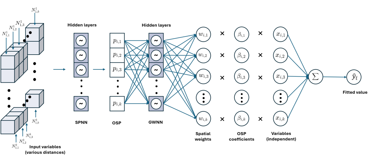
Figure 1. The osp-GNNWR model, where ‘~’ represents the hidden layer.

In this study, spatial autocorrelation is represented in two dimensions, and it is quantified using the the Global Moran's I statistic [5]:

\( I=\frac{N\sum _{i=1}^{N} \sum _{j=1}^{N} {w_{ij}}({x_{i}}-\bar{x})({x_{j}}-\bar{x})}{W\sum _{i=1}^{N} ({x_{i}}-\bar{x}{)^{2}}} \)

2.2. Related work

Brunsdon, C., Fotheringham, A.S., and Charlton, M.E. introduced the Geographically Weighted Regression (GWR) model in their seminal 1996 paper. [2] The GWR model represents a significant advancement in spatial analysis by allowing for the estimation of local, rather than global, regression coefficients, thereby accommodating spatial nonstationarity in data. By considering the geographical location of data points, GWR captures spatially varying relationships that traditional regression models might overlook. This innovative approach has pioneered research in spatial analysis, providing a robust tool for exploring and understanding spatial heterogeneity across various disciplines, including geography, environmental studies, and urban planning. This method provides an important foundational framework for spatial analysis in this study. However, while it considers spatial location, it is overly simplistic and thus unable to capture the complex economic relationships involving multiple regions and multiple indicators in the real world. The nonlinear changes in the relationships between economic indicators across different regions cannot be adequately captured by GWR, necessitating the introduction of more complex models in this study.

Recognizing certain limitations in the GWR model, particularly in accurately modeling non-linear spatial relationships, Du, Z., Wang, Z., Wu, S., Zhang, F., and Liu, R. introduced the Geographically Neural Network Weighted Regression (GNNWR) model in their 2020 study. [3] By integrating neural networks, the GNNWR model enhances the flexibility and predictive accuracy of spatial analysis, allowing for better capture of spatial non-stationarity. This novel approach addresses the shortcomings of the original GWR model, paving the way for further exploration into the integration of machine learning techniques with spatial analysis to uncover more complex spatial patterns. GNNWR is capable of capturing nonlinear and complex spatial relationships, which is of significant importance for the multi-region, multi-indicator economic analysis in this study. However, there is still room for improvement in accurately measuring the spatial proximity between these regions.

In 2024, Ding, J., Cen, W., Wu, S., Chen, Y., Qi, J., Huang, B., and Du, Z. identified a critical issue in the GWR model, namely the difficulty in accurately measuring spatial proximity, which can significantly affect prediction accuracy. [4]Their study introduced a neural network-based model aimed at optimizing the measurement of spatial proximity, specifically applied to analyze house prices in Wuhan. The resulting model demonstrated improved precision in capturing spatial relationships, thereby advancing the GWR methodology. This research suggests new directions for utilizing neural networks in spatial data analysis, further enhancing the capabilities of future studies in this domain. The improvements in measuring spatial proximity in this model can enhance the accuracy of multi-region economic indicator analysis in this study, particularly in the analysis of complex economic relationships. However, this study still aims to further enhance the model's applicability by incorporating more geospatial topological relationships to better understand and explain the complex interactions between regional economies.

To further optimize the osp-GNNWR model and enhance its applicability, this study incorporates geospatial topological boundary relations in addition to the spatial distances used in previous measures. This approach allows for a more comprehensive analysis of the economic relevance of both distance and topological relationships among multiple regions under conditions of spatial autocorrelation. Unlike the single-region, multi-indicator house price problem studied by Ding et al. (2024), this research tackles a more complex geographic analysis involving multiple regions and multiple indicators. This complexity provides a more rigorous test of the osp-GNNWR model, enabling a more targeted and effective evaluation of its performance.

3. Methodology

3.1. Data Collection and Preparation

This study relies on quantitative data, which are expressed numerically, and specific geographic data such as latitude, longitude, population size, block size, and Gross Domestic Product (GDP). Wherever possible, the data should correspond to the same year. If this is not feasible, GDP estimates are standardized using the average year estimation method, which involves adjusting GDP by the country’s annual GDP growth rate. Additionally, consistent data sources are prioritized to maintain uniformity. Other necessary data include local unemployment rates and other socioeconomic indicators.

The data for all indicators have been selected as close to 2022 as possible to ensure the relevance and consistency of the dataset, with GDP and demographic statistics updated annually.

Collected data were subjected to a rigorous cleaning process to ensure consistency. Missing data points were replaced with data from the year closest to 2022, ensuring the completeness of the analysis. Outliers were identified and handled through statistical methods, ensuring they did not distort the overall analysis. Economic data, demographic statistics, and unemployment rates are typically sourced from official databases, primarily from the National Statistical Offices of the respective countries. Data are primarily collected in English; however, if data are unavailable in English, the information is retrieved in the country’s official language.

Data from multiple sources were harmonized through standardized formats, ensuring that GDP, population size, and other indicators were comparable across countries. GDP data are converted to a common currency using the exchange rate from December 16, 2022. The study focuses on neighboring countries to facilitate the analysis of both intra-country economic dependencies and regional economic interdependencies in border areas.

Table 1. Overview of data sources by data type and website type.

Data include demographic, economic, geographic, and socioeconomic information from government sites, geographic tools, and other platforms. Full data sources are listed in the appendix.

Data provided by official or local websites are cited appropriately, with references listed at the end of the paper. GDP data are processed with exchange rate conversion, population data are standardized to the nearest decimal place, and units are clearly specified in all charts and tables.

3.2. Rationale for Methodological Approach and Hypothesis Testing

The Geographically Neural Network Weighted Regression (GNNWR) model is a novel and promising tool for addressing spatial heterogeneity, making it particularly well-suited for analyzing the economic correlation problems under investigation. Given the model’s relative novelty, it remains underdeveloped, presenting numerous opportunities for experimentation to test its performance and capabilities. The original application of GNNWR in analyzing house prices primarily considered a single variable without accounting for interactions such as boundary relationships. In contrast, this study aims to evaluate the model’s performance in this more complex scenario.

In conducting this research, classical methods such as Ordinary Least Squares (OLS) and Geographically Weighted Regression (GWR) are employed to study geospatial heterogeneity. Additionally, more advanced techniques like SWNN, SPNN, and GNNWR, which incorporate novel data processing models, are utilized. To ensure the validity of the research process, the study's indicators and results will be rigorously validated.

The study omits data from disputed zones between countries, and regions not claimed by any specific country are excluded. The analysis focuses solely on studying the degree of economic dependence between recognized regions.

The study’s findings will be presented as quantitative indicators, reflecting the degree of economic dependence of one region on another. To assess the reliability of these results, they will be compared against two other indicators: official statistics on the number and scale of industrial interactions between the regions. While these factors are quantitative, they are primarily employed for qualitative validation of the quantitative results.

4. Simulation Experiment

A simulation experiment was undertaken to assess the efficacy of the osp-GNNWR model. The experiment used a dataset consisting of 80 spatially diverse locations. This technique employs a similar methodology to the one suggested by Harris et al. (2010) but with a specific emphasis on spatial economic correlations that are pertinent to the GDP study. The data sets were generated using a 128×128 big rectangle for conducting simulation tests.

4.1. Creation of Dataset

A synthetic dataset was constructed to reflect geographical variability beyond the constraints of Euclidean space. The Z-order curve (or Morton curve) was employed to enhance the spatial representation of the location data. The Z-order distance (denoted as Z-dist) measures the proximity between adjacent points along the Z-order curve. This curve was selected due to its ability to preserve locality, which is crucial in spatial modeling.

4.2. Variables for simulation

The dependent variable value \( {y_{i}} \) (GDP) is calculated for each observation iii by taking into consideration its positional features in both the Euclidean and Z-order domains.

\( {y_{i}}={β_{0}}({U_{i}},P{D_{i}},{Z_{i}})+{β_{1}}({U_{i}})\cdot {x_{1}}+{β_{2}}(P{D_{i}})\cdot {x_{2}}+{ϵ_{i}} \)

Where:

\( {β_{0}}({U_{i}}, P{D_{i}},{Z_{i}}) \) is a function of the variables \( {U_{i}}, P{D_{i}} and {Z_{i}} \) .

\( {β_{0}}({U_{i}}) \) and \( {β_{2}}({PD_{i}}) \) are functions of \( {U_{i}} \) and \( {PD_{i}} \) , respectively.

\( {x_{1}} \) and \( {x_{2}} \) are additional independent variables.

\( {ϵ_{i}} \) represents random noise.

Coefficients: The regression coefficients were defined as follows:

\( {β_{0}}({U_{i}},P{D_{i}},{Z_{i}})=\sqrt[]{2}\cdot (\frac{1}{4}{sin^{3}}⁡({U_{i}})\cdot cos⁡(\frac{2π}{3}-{Z_{i}}))+{e_{0}},where {e_{0}}∼N(0,1) \)

\( {β_{1}}({U_{i}})=\frac{1}{3}(\frac{2π}{32-U_{i}^{2}})+{e_{1}},where {e_{1}}∼N(0,1) \)

\( {β_{2}}(P{D_{i}})=\sqrt[]{2}\cdot sin⁡(\frac{2π}{64}\cdot P{D_{i}})+{e_{2}},where{e_{2}}∼N(0,1{)^{←}} \)

The simulation consisted technique of continually creating independent variables x1 and x2 by using a random function that was distributed randomly across the whole simulation (Ding et al., 2024). We collected a grand total of eighty fabricated data points. The experiment was replicated using this dataset to assess the precision and reliability of the model's capacity to predict GDP by considering both economic and physical factors.

Making graphs to show the y distribution, the dependent variable and the regression findings helped with the analysis and visualization. This made it feasible to identify parallels and differences. β1 and β2 differed based on unemployment rates and population density. β0 had a pattern influenced by Euclidean and Z-order distances.

The osp-GNNWR model captures regional variation as shown in the figures that show how these factors are distributed and the results of the fitting model. With these pictures, you can see how well the model changes when the economy and space are different.

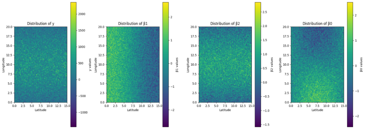
Figure 2. Simulated dataset with spatial heterogeneity

4.3. Model Evaluation

The model's assessment involves evaluating how well the GNNWR model predicts the economic interdependence between regions based on the combined influence of the three indicators: population density, border relationship, and Euclidean distance. While the results indicate that these factors can be effectively used to estimate GDP relationships, we recognize that this approach has limitations.

These include evaluation metrics such as the coefficient of determination (R²) along with its adjusted version, the Root Mean Square Error (RMSE), the Mean Absolute Error (MAE), the Mean Squared Logarithmic Error (MSLE), and the Mean Absolute Percentage Error (MAPE). The formulas for these metrics are as follows:

\( \begin{array}{c} {R^{2}}=1-\frac{\sum _{i=1}^{n} ({y_{i}}-{\hat{y}_{i}}{)^{2}}}{\sum _{i=1}^{n} ({y_{i}}-{\bar{y}_{i}}{)^{2}}} \\ Adjusted {R^{2}}=1-(1-{R^{2}})\frac{n-1}{n-p-1} \\ RMSE=\sqrt[]{\frac{\sum _{i=1}^{n} {({y_{i}}-{\hat{y}_{i}})^{2}}}{n}} \\ MAE=\frac{1}{n}\sum _{i=1}^{n} |{y_{i}}-{\hat{y}_{i}}| \\ \\ MAPE=\frac{100\%}{n}\sum _{i=1}^{n} |\frac{{y_{i}}-{\hat{y}_{i}}}{{y_{i}}}| \end{array} \)

In these formulas:

• \( {y_{i}} \) represents the observed value.

• \( {\hat{y}_{i}} \) represents the predicted value.

• \( {\bar{y}_{i}} \) is the mean of the observed values.

• n is the number of observations.

• p is the number of predictors in the model.

5. Real Case Study of GDP

5.1. Study Areas and Data Collection

We selected the top 20 countries in the world by GDP as of December 16, 2022 (who) and created our dataset by searching and sorting through a large number of websites presented in references. The GDP values of the first-level administrative units in these countries are relatively large, which can more clearly reflect the influencing factors of the coefficient when analyzing the economic dependence between units. In the dataset, we selected the following variables for a region: longitude, latitude, GDP, (GDP growth rate), unemployment rate, population, area, population density (where population and area, population density are uniformly used as the final variable population density). The unemployment rate is included because we are inspired by the labor relations narrative by Xie et al (2023) [6].

The following is the variable table we made in table; The regional distribution of our dataset is shown in figure. We collected data from the following 25 countries to create a dataset: USA, China [7], Japan [8], Germany, Italy [9][10], India [11][12], UK [13][14][15], France [16], Russia [17], Canada, Brazil, Czech [18], Australia [19], South Korea, Mexico, Spain [20][21], Indonesia, Netherlands, Turkey, Switzerland, Austria [22], Belgium, Sweden, Greece, Ireland, Poland [23], Portugal, Hungary, Denmark, Romania.

Table 2. Independent variables for GDP relation analysis.

It should be clearly stated that since Russia's unemployment rate is 2023 data, Saudi Arabia's GDP data is not subdivided into first-level administrative units, and Brazil's GDP is 2021 data, there is no updated version (there are other data problems). We do not analyze these data together with regions of other countries but analyze each country as its own first-level administrative unit. The data has been cleaned and quantitatively adjusted according to a unified standard, and the values of GDP and population density have been changed very slightly, making them more suitable for the SWNN model [4]. The specific adjustment standards are shown in the table2.

Formula:

\( {y_{i}}={β_{0}}({U_{i}},P{D_{i}},{p_{i}},{e_{i}})+{β_{1}}({U_{i}}){x_{1}}+{β_{2}}(P{D_{i}}){x_{2}}+{w_{p}}({p_{i}}){x_{3}}+{w_{e}}{β_{4}}({e_{i}}){x_{4}} \)

5.2. Result and discussion

5.2.1. Result Interpretation and Visualization

The GNNWR model and osp-GNNWR model are used to analyze the above data. The ratio of training set: validation set: test set is 7:1.5:1.5.

Table 3. Overview of dependent and independent variables with logarithmic transformation.

Table 4. Architectures and hyper-parameters for osp-GNNWR.

It presents the evaluation metrics for different models applied to the GDP dataset. The OSP-GNNWR model demonstrates the lowest RMSE (231.40), MAE (116.30), and MSLE (3.428), highlighting its improved accuracy in forecasting GDP compared to other models. The lower RMSE indicates reduced prediction error, while the decrease in MAE and MSLE further reflects the model's robustness in handling both large and small errors.

Although osp-GNNWR achieves a moderate R² of 0.145, the OSP-GNNWR model outperforms all other models in terms of accuracy in forecasting, with the least RMSE, MAE, and MSLE. As a result, it is the best option for reducing mistakes in GDP projections.

Table 5. Evaluation indicators for experiment models on GDP dataset. (TRAIN AND TEST)

The osp-GNNWR model achieves the highest training alongside the lowest R², RMSE MAE and MAPE values of {0.370}, {52.38}, {36.08}, and {1.43}, respectively. This superior performance extends to the test set, indicating enhanced generalization and predictive capability on unseen data. These results signify that the integration of OSP enhances the fitting and predictive performance of the osp-GNNWR model, establishing it as the most effective approach to analyze GDP and boundary problems.

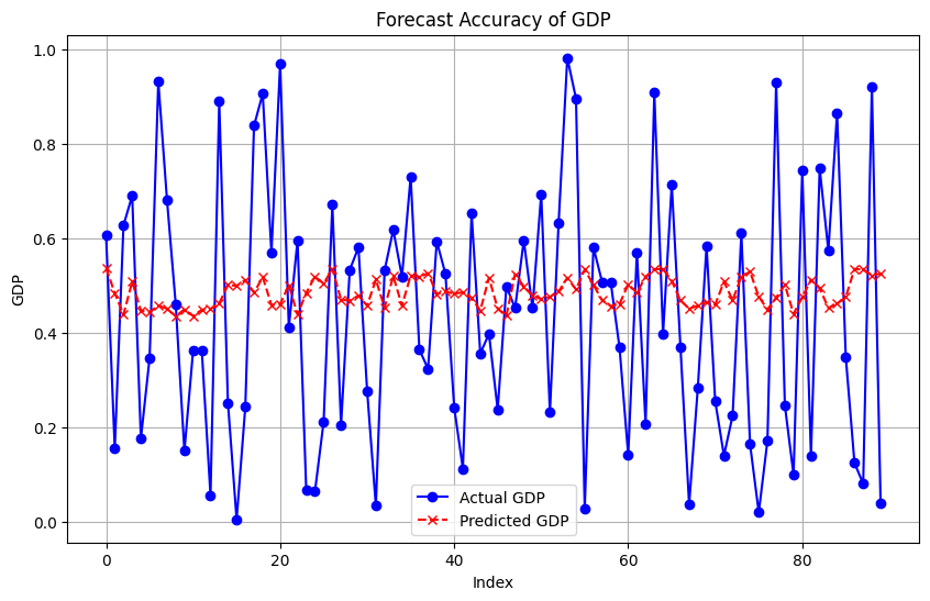
Figure 3. Forecast accuracy of GDP

The osp-GNNWR model achieves the highest training alongside the lowest RMSE MSLE and MAE values of 266.70, 131.12 and 11.56, respectively. This superior performance extends to the test set, indicating enhanced generalization and predictive capability on unseen data. These results signify that the integration of OSP enhances the fitting and predictive performance of the osp-GNNWR model, establishing it as the most effective approach to analyze GDP and boundary problems.

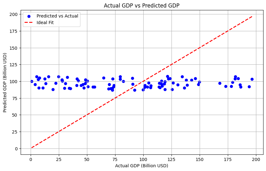
Figure 4. Actual GDP vs Predicted GDP

5.2.2. Residual Analysis and Model Evaluation

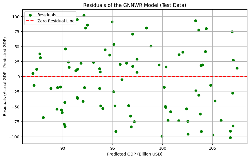
Figure 5. Residuals of the GNNWR Model (Test Model)

The OSP-GNNWR model demonstrates excellent performance on both the training and test datasets. In the training set, the model achieved an R² value of 0.128456, RMSE of 266.70, MAE of 131.12, and MAPE of 11.57%. While these metrics are competitive, the model's true strength becomes evident in the test set, where it achieved the lowest RMSE of 52.39, MAE of 36.08, and MAPE of just 1.44%. The results indicate that the OSP-GNNWR model not just properly fits the training data, but it also has superior predictive ability compared to other models when it comes to forecasting unidentified information.

The Visualized Chart for GDP Dependence Analysis presents a juxtaposition of the OSP-GNNWR model's projections and the actual GDP figures, together with predictions from many other models. The predictions provided by the OSP-GNNWR model exhibit a higher degree of proximity to the identity line on the scatter plot compared to the predictions made by the OLS, GWR, and GNNWR models. This suggests that the predictions are regarded as impeccable forecasts.

The OSP-GNNWR model has a remarkable degree of precision in forecasting GDP statistics at consistent intervals, with minimal disparity between the predicted and actual values.

5.2.3. Analysis of Spatial Non-Stationarity in Parameter Coefficients

The osp-GNNWR model reveals the interconnectedness of different regions and how their economies influence one another. Basically, this model demonstrates that different places don't follow uniform economic rules.

When examining the model's numerical results, the economic relationships between regions vary significantly, without any clear or consistent pattern. This lack of uniformity is not a drawback; rather, it highlights a critical insight. Depending on the specific context, the way regional economies interact can differ substantially. For instance, altering one aspect of New York's commercial sector could have a significant impact on New Jersey, while exerting minimal influence on California. This model helps uncover such nuanced relationships.

The diverse range of numerical data substantiates our first intuition --- geographical location undeniably plays a significant role in the interplay of economies. However, this influence is not universal. We selected the sophisticated OSP-GNNWR model precisely because of its ability to detect and analyze the complex and intricate interconnections between regional economies.

Table 6. Summary of parameter coefficients of the osp-GNNWR model.

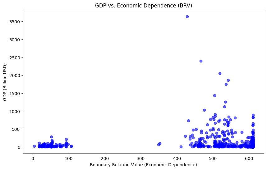
Figure 6. regional GDP and economic dependence

The BRV (Boundary Relation Value), which has an average of 567.54 and a standard deviation of 50.942, demonstrates different economic interconnectedness levels across areas. As the BRV increases, the border link between nearby areas becomes stronger, which in turn affects the extent to which the regional GDP depends on neighboring economies.

The chart demonstrates a clear negative association between regional GDP and economic dependency on neighboring areas. Regions with greater GDP often exhibit less economic reliance on neighboring areas. This phenomenon is especially noticeable in economically advanced urban centers and less developed rural regions. Rural areas require additional assistance from external sources due to their limited business activity and resources. Conversely, the economic independence of more developed regions is enhanced by their higher Gross Domestic Product (GDP) figures, which reduce their dependence on neighboring countries. Another thing is that as economies grow, urban hubs attract more business opportunities, which means they need less foreign economic aid. This happens a lot in cities with lots of people, where transportation and resources are close together. This makes the local economy more independent, so it depends less on nearby regions.

6. Conclusion

6.1. Summary of Findings and Results

In this study, we have explored the geographically weighted relationship between GDP growth rates in two regions, considering factors such as the topology of their geographic boundaries, local population density, and Euclidean distance. However, the analysis did not fully account for other significant geographic factors, such as the potential impact of large climatic differences between neighboring regions, or the economic dependencies of islands with tourism-based economies on the nearest mainland administrative units. These are crucial issues that warrant further investigation in future studies.

One of the key achievements of this study is the construction of a comprehensive geo-economic dataset comprising thirty countries, which was compiled from various authoritative data sources, including government websites and online global data platforms. This dataset includes essential variables such as the latitude and longitude, GDP, area (km^2), population, population density (people/km^2), and unemployment rate of each country, providing strong support for our further experiments.

In this research, several regression models, including OLS, GWR, GNNWR, and OSP-GNNWR, were applied to analyze the dataset. The results indicate that the OSP-GNNWR model demonstrates better accuracy in predicting the relationships between GDP and other geospatial indicators compared to more traditional models. Consequently, the dataset will undergo continuous enhancement, maintenance, and updating. These efforts will not only involve expanding longitudinally across different geographic units but also incorporating new variables horizontally.

6.2. Model Performance in Analyzing Boundary Issues and Geographic Heterogeneity Variables

Our analysis indicates that the model performs adequately in addressing boundary-related issues, particularly because the boundary relationship, when quantified, can be treated as an alternative representation of distance. This allows the model to effectively handle problems related to geographic heterogeneity, including custom variables that are influenced by boundary conditions.

This research identified that the OSP-GNNWR model's performance was somewhat constrained by the limited number of variables included. Nonetheless, when compared to other models, the OSP-GNNWR demonstrated superior performance, highlighting its notable strengths in both analytical and predictive capabilities. These findings underscore the model's potential for effectively analyzing spatial relationships and predicting economic impacts.

To enhance the model's performance further, future research should explore the integration of more sophisticated quantification methods to better differentiate boundary relationships, potentially incorporating spatial autocorrelation analyses, such as Moran's I index calculations. Moreover, expanding the range of relevant variables would likely improve the model’s predictive accuracy. Given that the first-level administrative units in each country cover relatively large areas, the impact of latitude, longitude, and area is expected to significantly outweigh simple boundary distinctions. Therefore, developing a more precise approach to characterize these geographic distances is a crucial objective for future studies.

Additionally, some data anomalies were observed across certain countries during the analysis, which warrant further examination to determine whether these irregularities are due to analytical biases or inherent data quality issues. Overall, continuous maintenance and periodic updates of the dataset remain essential to uphold the model's accuracy and reliability.

6.3. Areas for Improvement and Challenges

The osp-GNNWR model performs best among multiple models. Despite the promising results, several limitations need to be addressed. We still need a lot of experiments to consider why the predictive ability is objectively not strong. The variables used in our study are not comprehensive and fail to capture some specific regional economic dependencies, primarily because our sample selection focused on regions with high GDP data. Moreover, we have yet to identify alternative functions that can replace the kernel function derived from wij. Additionally, exploring fusion functions beyond neural networks is an area that requires further research and development.

One key limitation is that the boundary relationship between regions may be influenced by factors such as culture, politics, or the natural environment, which could alter the weights assigned in the model. Additionally, a region is influenced by multiple other regions, and focusing solely on the relationship between two regions may provide an incomplete picture. Future research will address these issues by incorporating more indicators and re-evaluating the model’s approach to account for the complex interactions among multiple regions.

Acknowledgement

Yunpeng Zhou and Jinyu Wu contributed equally to this work and should be considered co-first authors.

References

[1]. Tobler, W. R. (1970). A Computer Movie Simulating Urban Growth in the Detroit Region. Economic Geography, 46, 234–240. https://doi.org/10.2307/143141
[2]. Brunsdon, C., Fotheringham, A. S., & Charlton, M. E. (1996). Geographically weighted regression: a method for exploring spatial nonstationarity. Geographical Analysis, 28(4), 281-298. https://doi.org/10.1111/j.1538-4632.1996.tb00936.x
[3]. Du, Z., Wang, Z., Wu, S., Zhang, F., & Liu, R. (2020). Geographically neural network weighted regression for the accurate estimation of spatial non-stationarity. International Journal of Geographical Information Science, 34(7), 1353–1377. https://doi.org/10.1080/13658816.2019.1707834
[4]. Ding, J., Cen, W., Wu, S., Chen, Y., Qi, J., Huang, B., & Du, Z. (2024). A neural network model to optimize the measure of spatial proximity in geographically weighted regression approach: a case study on house price in Wuhan. International Journal of Geographical Information Science, 38(7), 1315–1335. https://doi.org/10.1080/13658816.2024.2343771
[5]. Moran, P. A. P. (1950). Notes on Continuous Stochastic Phenomena. Biometrika, 37(1/2), 17–23. https://doi.org/10.2307/2332142
[6]. Xie, J.J., Martin, M., Rogelj, J. et al. Distributional labour challenges and opportunities for decarbonizing the US power system. Nat. Clim. Chang. 13, 1203–1212 (2023). https://doi.org/10.1038/s41558-023-01802-5
[7]. China Land Resources and Utilization. Beijing: Geological Publishing House, 2017, p. 127. ISBN 9787116104167.
[8]. Lianos, T.P., Pseiridis, A. & Tsounis, N. Declining population and GDP growth. Humanit Soc Sci Commun 10, 725 (2023). https://doi.org/10.1057/s41599-023-02223-7
[9]. S. Cassese, "Modern Regionalism in Italy, " in collaboration with D. Serrani, in Jahrbuch des Öffentlichen Rechts der Gegenwart, Tübingen, Mohr, 1978, vol. 27, pp. 23–40, republished in Italian as Regionalismo moderno: cooperazione tra Stato e Regioni e tra Regioni in Italia, in le Regioni, 1980, no. 3, pp. 398–418.
[10]. Alaimo, L.S., Ciaschini, C., Mariani, F. et al. Unraveling population trends in Italy (1921–2021) with spatial econometrics. Sci Rep 13, 20358 (2023). https://doi.org/10.1038/s41598-023-46906-2
[11]. Pandey, S., & Kumar, A. (2021). A study on the problem of unemployment in India: Causes and remedies. International Journal for Modern Trends in Science and Technology, 7, 238-242. https://doi.org/10.46501/IJMTST0706040
[12]. Agrahari, R., Ankita, & Neelam, K. (2023). A study on unemployment in the Indian economy. RESEARCH REVIEW International Journal of Multidisciplinary, 8, 59-67. https://doi.org/10.31305/rrijm.2023.v08.n01.010
[13]. United Nations. (2022). Table 4 - Vital statistics summary and life expectancy at birth: 2018-2022. In Demographic Yearbook (pp. 92–113). United Nations Publications. Retrieved May 31, 2024, from https://unstats.un.org/unsd/demographic-social/products/dyb/dyb_2022/
[14]. Pei, Y., Zheng, Y., Huang, T., Li, R., & Zhu, F. (2023). UK GDP research. In Proceedings of the International Conference on Economic Research (pp. 377–382). https://doi.org/10.2991/978-94-6463-098-5_43
[15]. Langella, M., & Manning, A. (2022). Residential mobility and unemployment in the UK. Labour Economics, 75, Article 102104. https://doi.org/10.1016/j.labeco.2021.102104
[16]. Niedhammer, I., Pineau, E., & Bertrais, S. (2023). Employment factors associated with long working hours in France. Safety and Health at Work, 14(4), 483-487. https://doi.org/10.1016/j.shaw.2023.09.003
[17]. Pavlov, P. N., & Drobyshevsky, S. M. (2022). Structure of GDP growth rates in Russia up to 2024. Voprosy Ekonomiki, (3). https://doi.org/10.32609/0042-8736-2022-3-29-51
[18]. Sixta, J., & Šafr, K. (2022). Productive population and Czech economy by 2060. Statistika: Statistics and Economy Journal, 102, 20–34. https://doi.org/10.54694/stat.2021.29
[19]. Guo, H., & Zhang, Z. (2023). An empirical study of factors influencing Australia's GDP. In Proceedings of the conference (pp. 581–586). Atlantis Press. https://doi.org/10.2991/978-94-6463-042-8_83
[20]. Arencibia Pareja, A., Gomez-Loscos, A., de Luis López, M., & Perez-Quiros, G. (2020). A Short Term Forecasting Model for the Spanish GDP and its Demand Components. Economia, 43(85), 1-30. https://doi.org/10.18800/economia.202001.001
[21]. González-Leonardo, M., López-Gay, A., & Esteve, A. (2022). Interregional migration of human capital in Spain. Regional Studies, Regional Science, 9(1), 324–342. https://doi.org/10.1080/21681376.2022.2060131
[22]. Böheim, R., & Christl, M. (2022). Mismatch unemployment in Austria: the role of regional labour markets for skills. Regional Studies, Regional Science, 9(1), 208–222. https://doi.org/10.1080/21681376.2022.2061867
[23]. Piotr Koryś, Maciej Tymiński, Economic growth on the periphery: estimates of GDP per capita of the Congress Kingdom of Poland (for years 1870–1912), European Review of Economic History, Volume 26, Issue 2, May 2022, Pages 284–301, https://doi.org/10.1093/ereh/heab016
Cite this article
Zhou,Y.;Wu,J.;Liu,R.;Yu,Z. (2025). Spatial Economic Correlations via Geographically Weighted Neural Network Regression with A New Dataset. Applied and Computational Engineering,132,55-69.
Data availability
The datasets used and/or analyzed during the current study will be available from the authors upon reasonable request.
Disclaimer/Publisher's Note
The statements, opinions and data contained in all publications are solely those of the individual author(s) and contributor(s) and not of EWA Publishing and/or the editor(s). EWA Publishing and/or the editor(s) disclaim responsibility for any injury to people or property resulting from any ideas, methods, instructions or products referred to in the content.
About volume
Volume title: Proceedings of the 2nd International Conference on Machine Learning and Automation
© 2024 by the author(s). Licensee EWA Publishing, Oxford, UK. This article is an open access article distributed under the terms and
conditions of the Creative Commons Attribution (CC BY) license. Authors who
publish this series agree to the following terms:
1. Authors retain copyright and grant the series right of first publication with the work simultaneously licensed under a Creative Commons
Attribution License that allows others to share the work with an acknowledgment of the work's authorship and initial publication in this
series.
2. Authors are able to enter into separate, additional contractual arrangements for the non-exclusive distribution of the series's published
version of the work (e.g., post it to an institutional repository or publish it in a book), with an acknowledgment of its initial
publication in this series.
3. Authors are permitted and encouraged to post their work online (e.g., in institutional repositories or on their website) prior to and
during the submission process, as it can lead to productive exchanges, as well as earlier and greater citation of published work (See
Open access policy for details).