1. Introduction

There are hundreds of millions of clusters in the universe, and we can get pictures of clusters through various detectors. But usually, these clusters are merged because they are too dense, which makes them look as a whole. So, we need a detector program to help us calculate the number of clusters in a picture, their exact location, and the exact cluster center mass.

In this experiment, we need to complete a small cluster-finding test with a set of data provided by the professor. The first line of the data shows the total number of clusters in each group. The second to eleventh line are the real center mass of each cluster and a 64*64 data set (Figure 1) that contains the data of the 10 clusters. We have a total of 1000 data sets, each with a fixed number of 10 clusters, and our goal is to identify the number of clusters in each set and make our predicted center mass match the real center mass as closely as possible. Our technical challenge is that we cannot tell the program how many in each graph of the clusters in each group, but to allow the computer pass algorithm to identify exactly 10 clusters in each group on its own. if there are many overlapping clusters in a set of graphs, then the program may identify fewer than 10 clusters, which is the subsequent problem that needs to be solved. Finally, even though the computer can identify 10 clusters, it still needs to find the center mass of the clusters accurately; in some cases, the highest number does not represent the center mass, and some high numbers might appear when two clusters overlap. Therefore, we need to find a series of ways to make the computer find the most accurate solution without knowing the actual data.

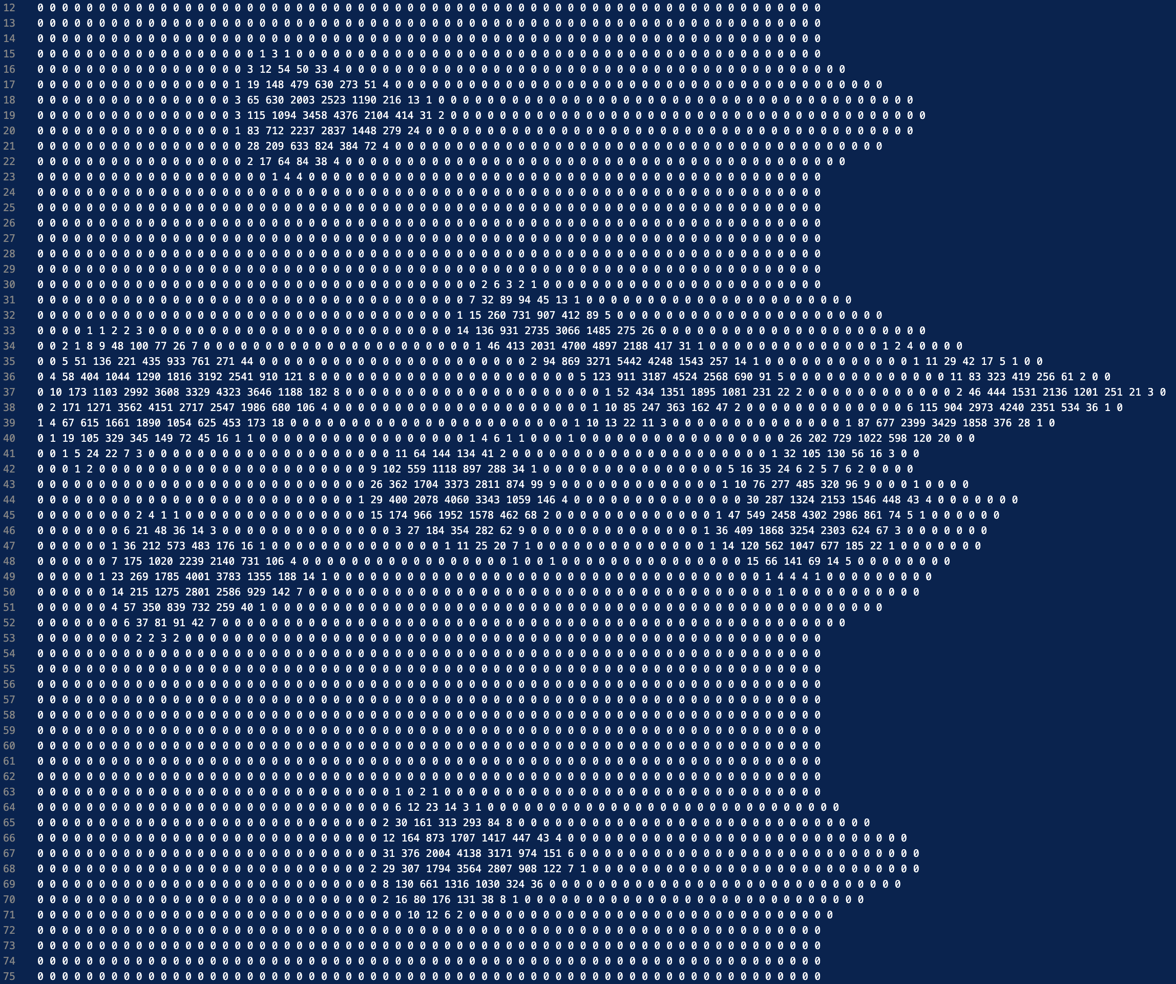
Figure 1. a 64*64 dataset for example

Cluster finding in data analysis has been an active field of research over the past several decades, with algorithms developed to extract groups or “clusters” from complicated datasets. The most common methods include k-Means and hierarchical clustering, but recently new machine learning-based approaches have been proposed to provide higher accuracy levels with lower computational costs.

Despite its simplicity and effectiveness, k-Means clustering still remains one of the most frequently used algorithms. On the flip side, it is very sensitive to where you initially place your cluster centers and can have a hard time with noisy or overlapping data. Many enhancements to the original k-Means were suggested by researchers. For example, Ran et al. [1] introduces a noise-resistant k-Means variant tailored to the task of urban hotspot detection, which enhances cluster quality by accounting for noisy data points using an additional noise algorithm. Ikotun et al. [2] provided a thorough review of possible k-Means variants for large-scale datasets, discussing advanced initialization techniques, distance measures, and optimization strategies to address limitations in the standard algorithm. Additionally, Govender and Sivakumar [3] demonstrated that k-Means clustering is useful for analyzing air pollution data, especially when combined with hierarchical methods; substantial improvements in cluster interpretation can be achieved alongside accuracy.

In practice, many other cluster-finding methods have been developed to solve the challenges presented in various domains beyond k-Means. Yantovski-Barth et al. introduced the CluMPR algorithm, a new method for detecting galaxy clusters in astronomical surveys. Their method integrates different data sources using a hybrid machine learning and statistical approach to increase detection accuracy and reliability. In the medical field, Chen-xi et al. [4-5] used clustering algorithms to analyze clinical and CT data related to COVID-19 patients, demonstrating the potential of clustering techniques in finding patterns in medical datasets and providing insights into disease spread dynamics.

Our work extends previous research by combining different methods like Local Max, k-Means, and Convolutional Neural Networks (CNNs) to overcome certain drawbacks identified in earlier studies. Local Max provides a simple but efficient heuristic to identify reliable cluster centers, which k-Means can refine by iteratively moving data points closer to their best possible center. We also apply state-of-the-art deep learning techniques, including CNNs combined with average pooling and center-of-gravity calculations, to solve datasets containing complex, noisy data with overlapping clusters. By combining traditional and modern approaches, we aim to improve the robustness and accuracy of cluster detection, offering a more flexible solution applicable to fields as diverse as astronomy, urban planning, or medical diagnostics.

Our method harnesses both traditional and more recent algorithms, seeking to exploit their complementary strengths while mitigating their individual drawbacks, providing a comprehensive solution for accurate cluster discovery across diverse datasets.

2. Analysis of Local maximum and k-Means Algorithms

In many computer vision tasks where image data processing and analysis is required, accurate identification of cluster centers (known as centroids), becomes heavily important to execute essential operations like clustering. There are similar such methods that can help us locate the centroids of clusters accurately to name a few, in this dataset we used local maximum & k means algorithm [2]. This will help to achieve better accuracy for cluster detection and center localization. Above, an explanation by referencing to the data points of Figure 2 how each algorithm based on which principles and in what form this application takes place is presented.

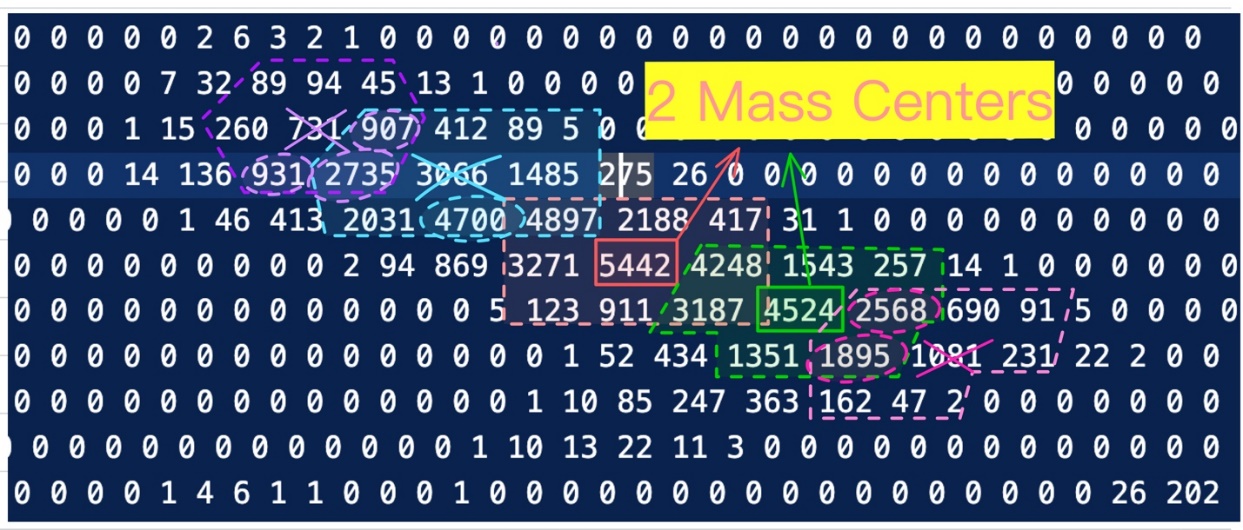
Figure 2. dataset with 2 mass centers.

2.1. Local Maximum Analysis

Local maximum is a simple algorithm for finding local maxima in an ordered collection of data points. The basic idea behind this approach is to look at each pixel with respect to its local neighborhood and test if it belongs there as implying a local maximum (which means that the current pixel might be considered in future as a cluster center) or not. The Local maximum method identifies these local maxima as candidate cluster centroids in our data set, shown is Figure 2.

2.1.1. Data Initialization and Neighborhood Definition

We begin with the given two-dimensional data set (a matrix representing pixel intensities). The data matrix in Figure 2 is an 11x11 grid, with values ranging from 0 to 5442, where each value represents the brightness or intensity of a pixel in the image. The first step in the Local maximum algorithm is to define the neighborhood of each point [4]. In this example, a 3x3 neighborhood is utilized (illustrated by the yellow box in Figure 2). For instance, consider the data point 2735 (highlighted by a purple dashed line); its neighborhood consists of the following points: 136, 931, 906, 1485, 3966, 2031, 4700, 2188.

2.1.2. Identifying Local Maxima

For each pixel, such as 2735, we compare its value against all its neighboring points. If the current pixel's value is greater than all its neighbors, it is marked as a local maximum. In Figure 2, the data point 4524 is identified as a local maximum because it has the highest value within its neighborhood (green dashed box). Conversely, the point 2735 is not the maximum within its neighborhood, so it is not marked as a local maximum.

2.1.3. Marking Initial Cluster Centers

Once local maxima are identified, these points are marked as initial cluster centers. In Figure 2, 4524 and 5442 are marked as initial potential cluster centers since they are local maxima. The advantage of the Local maximum algorithm is that it quickly identifies prominent high-intensity regions in the data, which serves as a good starting point for subsequent optimization.

2.2. Analysis of the k-Means Algorithm

The k-Means algorithm is an iterative clustering method that aims to adjust the positions of cluster centers by minimizing the squared distance from the points to their nearest cluster center. The strength of the k-Means algorithm lies in its ability to refine the initial cluster center positions provided by the Local maximum method to achieve a more accurate representation of the data's overall distribution.

2.2.1. Initialization of Cluster Centers

In our case, the k-Means algorithm begins by using the local maxima identified by the Local maximum method (4524 and 5442 in Figure 2) as the initial cluster centers. These points represent the most likely locations for the centers of the clusters, which the k-Means algorithm will further optimize.

2.2.2. Calculating the Distance from Each Point to Cluster Centers

Next, for every point in the data set, the algorithm calculates its distance to each cluster center. For example, the distance from point 2735 to cluster centers 4524 and 5442 is computed as follows:

\( Distance=\sqrt[]{{({x_{2}}-{x_{1}})^{2}}+{({y_{2}}-{y_{1}})^{2}}} \)

\( {Distance_{3187→5442}}=\sqrt[]{{(5-3)^{2}}+{(4-5)^{2}}}=\sqrt[]{4+1}=\sqrt[]{5}≈2.236 \)

\( {Distance_{3187→5442}}=\sqrt[]{{(5-7)^{2}}+{(4-7)^{2}}}=\sqrt[]{4+9}=\sqrt[]{13}≈3.605 \)

2.2.3. Updating Cluster Center Positions

After all data points are assigned to the nearest cluster centers, the algorithm calculates the weighted average position of every point in specific clusters. Update the cluster center to be this weighted average. An example could be the cluster where centroid 4524 belongs (green area) made up of points such as 3187, 1351, and so on. The new cluster center is calculated as:

\( New Center=\frac{\sum (coordinates of all points)*weights}{total weight} \)

2.2.4. Iterating Until Convergence

The k-Means algorithm goes back to calculating the distance between points and centers, then updates the center positions until they remain relatively stable, which indicates convergence. This process repeats until the cluster centers are in their optimal positions regarding the data.

We have talked about the situation of dataset which contains one and two mass centers. We could see that our local max and k-Means algorithm could handle them pretty good. But what if the condition got more complex? Will this method still work? One of the most featured datasets is number 292 dataset. It has 7 clusters next to each other and one pair of them heavily overlapping. At this situation, this algorithm will mistakenly identify the overlapped clusters as one mass center.

3. Approach through the Convolutional Neural Network

3.1. Introduction of CNN

Convolutional neural network (CNN) is a deep learning model based on Pytorch. This learning model is generally used to process and analyze data with grid-like topologies such as images. A man named Yann LeCun first proposed the concept of CNN in the late 1980s. The basic principle of CNN is to apply a set of learnable filters (cores) to the input data using convolutional layers, ultimately enabling the model to automatically capture spatial layers and patterns in the image data to define the image.[6]

CNN is composed of three layers, including convolutional layer, pooling layer and fully connected layer. The function of the convolutional layer is to perform core operations by sliding filters over the input data and detect pattern features such as edges and textures. The pooling layer reduces the spatial dimension of the data, which helps to control overfitting and reduce computational complexity. The fully connected layer is typically located at the end of the network and is often used to integrate extracted features to perform the final classification or regression task.

3.2. How it works in this project

In this project, convolutional neural networks (CNN) were used to predict the number and location of clusters in 1000 images. The CNN model trains the sample to predict the number of clusters and the coordinates of their centers. The model (Figure 3) consists of three convolution layers, with additional batch normalization layer, pool layer and fully connected layer. The entire CNN model extracts feature from the input images and learns patterns related to the number of clusters and their location.[7]

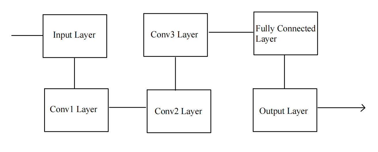
Figure 3. Simple diagram of CNN structure

During the training process, a custom loss function was added. This custom loss function combines mean square error (MSE) with cluster center coordinates to predict the number of clusters and optimize the model. The training process involves feeding batch data into the model, which is controlled by batch size parameters. The batch size determines the number of samples to be processed in the dataset before updating the model weights. It plays a key role in balancing training speed and memory use as well as stabilizing the learning process. [8][9]

\( Loss={MSE_{clusters}}+{MSE_{centroids}} \)

\( {MSE_{centroids}}=\frac{1}{N}\sum _{i=1}^{N}\sum _{j=1}^{K}({\hat{y}_{i,j}}-{y_{i,j}}) \)

\( {MSE_{centroids}}=\frac{1}{N}\sum _{j=1}^{N}{({\hat{y}_{i,clusters}}-{y_{i,clusters}})^{2}} \)

The code also adds an early stop mechanism. The early stop mechanism works by forcing training to stop if the verification loss does not improve within a specified number of epochs. The early stop mechanism can prevent overfitting to some extent. At the same time, the model uses a separate validation set and calculates validation losses, which ensures that the model generalizes well to previously unseen data.

Finally, the performance of the model in predicting cluster positions through image data is evaluated by comparing the trained predicted cluster positions with the actual cluster positions. The evaluation criteria include calculating the standard deviation (std) of the difference between the prediction and the actual clustering center to provide a measure of the model's accuracy. And the results are visualized with a histogram that concisely shows the distribution of errors in the x and y directions and the overall error in the clustering position.

3.3. What challenge we encounter

In the process of using CNN to detect the number of image clusters, two serious problems and challenges have been discovered. First, we observed that validation losses were significantly higher than training losses, indicating a potential overfitting problem. Typically, overfitting occurs when the model is too focused on learning training data, capturing noise and irrelevant details rather than general patterns. This is often due to overly complex models or inadequate regularization, resulting in models that perform well on training data but poorly on previously unseen validation data. In this case (Figure 4), the difference between training and validation losses indicates that the model only remembers the training data, rather than learning broadly, resulting in poor performance on the new data.

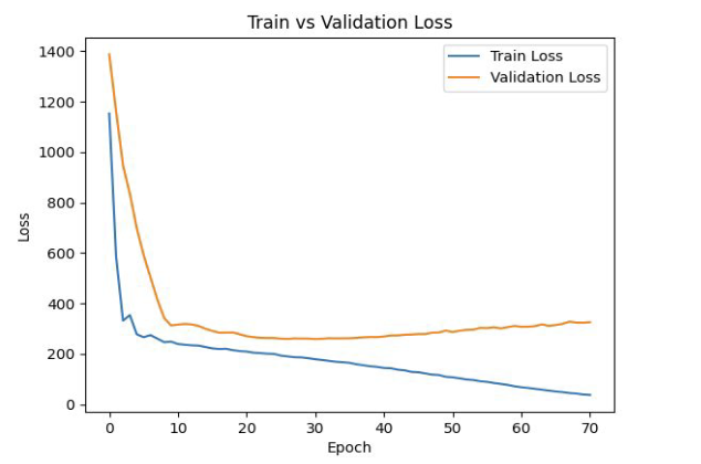
Figure 4. Train loss v.s Validation loss

Second, the dataset used for training contains 1,000 images, with exactly 10 clusters per image. This homogeneity in the training data raises concerns about the ability of the model to generalize to images with different numbers of clusters. Because the model is only exposed to and trained on images with 10 clusters, when it is used in the future to look at images with an uncertain number of clusters, it may be difficult to accurately predict the number of clusters in images with different cluster numbers. This limitation leads to unreliable predictions when applied to more diverse datasets, where the number of clusters is not fixed. The generalization ability of the model is critical to its practical application, and the lack of diversity in the training data poses a major challenge to achieving robustness.

4. Average Pooling & Center of Gravity

Average pooling is a commonly used pooling technique in machine learning and computer vision. Based on PyTorch, it serves to reduce the number of parameters and computational load while preserving key information in the feature maps.

The average pooling method consists of three steps. The feature map is first divided into several non-overlapping local regions, known as kernels. Next, for each kernel, the mean value of all elements within that region is calculated, as shown below [10]:

\( {f_{AP}}(x)=\frac{1}{n}\sum _{i=1}^{n}{x_{i}} \)

Finally, each average value becomes the value at the position of the kernel in the pooled feature map. Through the above process, a smaller-sized feature map is obtained, which contains the key information from the original feature map.

In this project, our group also tried to employ average pooling method to find clusters in the graphs. We set the kernel size to 3 while using average pooling method. To eliminate the noise in the graph that may interfere with the prediction of centers of clusters, we set a threshold that equals 0.6 times of the maximum of grayscale values in the graph. After we use average pooling, there are fewer bright pixels, yet we still have to eliminate some of them that are actually not centers. Thus, in the next step, we use the center of gravity, where we calculate the weighted average of the bright pixels next to each other in the pooled graphs, and use it as the predicted center of the cluster. This method is also able to predict the number of clusters in each graph. Then, we utilize Hungarian method to match the real centers of clusters and predicted ones. This algorithm aims at matching them in pairs, so that the sum of the distance of two points in a pair is the smallest. [11][12]

With this method, 862 graphs are predicted to have 10 clusters out of 1000 graphs, better than 789 graphs in the first approach.

Figure 5 shows the real centers of clusters (yellow cross) and predicted centers of clusters (red cross) of graph 55. We can find that when a cluster is isolated, it predicts quite well; on the contrary, when two or more clusters are next to each other, there are usually intervals between predicted centers and real centers. The distance between two predicted centers is usually smaller than the distance between the two real centers.

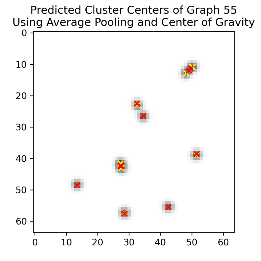
Figure 5. Predicted cluster centers of graph 55 using average pooling

The standard deviation is about 0.319, while distance of matched centers (dr) ranges from 0 to 2.06. Both the standard deviation and the maximum of dr is smaller than those in the first method. The distribution of dr is shown below in Figure 6.

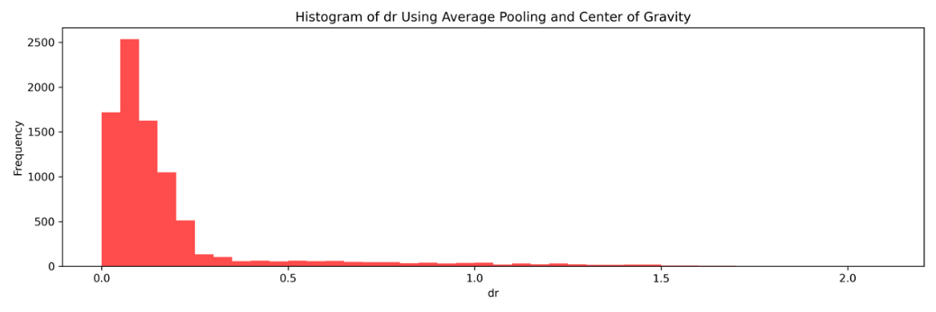
Figure 6. Histogram of dr using center of average pooling

The following picture (Figure 7) is the distribution of dr in the range 0 to 0.5, where we can see that most of dr falls between 0 to 0.25, while the peak frequency is between 0.06 and 0.07.

Figure 7. Histogram of dr in range [0, 0.5] using average pooling

5. Average Pooling, Center of Gravity & k-Means

The previous method yields better results than the first two methods, yet it still has problems when dealing with the clusters that are near each other. We have mentioned that the distance between two predicted centers is usually smaller than the distance between the two real centers. The main problem happens during the calculation of center of gravity method. In this algorithm, the way to identify predicted centers is as follows: draw a circle with a radius of 3 around a bright pixel and calculate the weighted average of all the bright pixels in the circle. As a result, some pixels between the predicted centers are calculated more than once. Nevertheless, these pixels are actually influenced by two or more clusters; in other words, the values of these pixels are sums of two or more numbers. Consequently, we have to add some algorithm so that all of these pixels are only calculated once when finding centers. Under this circumstance, k-Means method may become a good approach, since we have identified the number of clusters in each graph. We use the predicted center of clusters as the initial centroids, and classify the pixels into 10 clusters, while calculating the predicted center of each cluster. Then, we utilize Hungarian method again to match the real centers of clusters and predicted ones.

Figure 8 shows the real centers of clusters (white dot) and predicted centers of clusters (red dot) of graph 55. We can find that when a cluster is isolated, it still predicts well; meanwhile, when two or more clusters are next to each other, the intervals between predicted centers and real centers are much smaller than before.

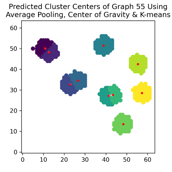
Figure 8. Predicted cluster centers of graph 55 using average pooling and k-Means

The standard deviation is about 0.0566, while dr ranges from 0 to 0.63. Both the standard deviation and the maximum of dr is smaller than before. The distribution of distance of matched centers (dr) is shown below in Figure 9.

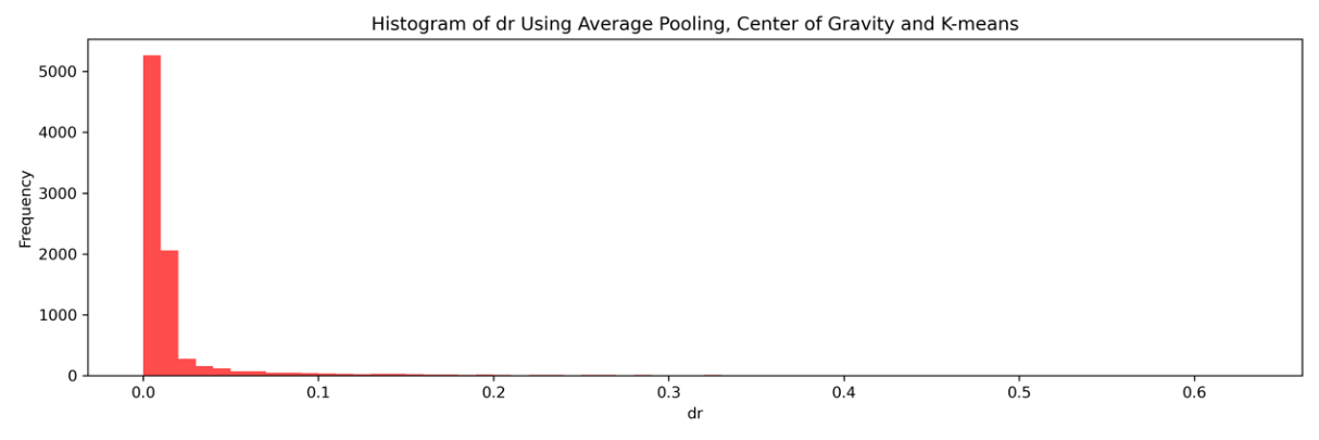
Figure 9. Histogram of dr using average pooling and k-Means

Figure 10 is the distribution of dr in the range 0 to 0.1, where we can see that most of dr falls between 0 to 0.02, while the peak frequency is between 0.004 and 0.006.

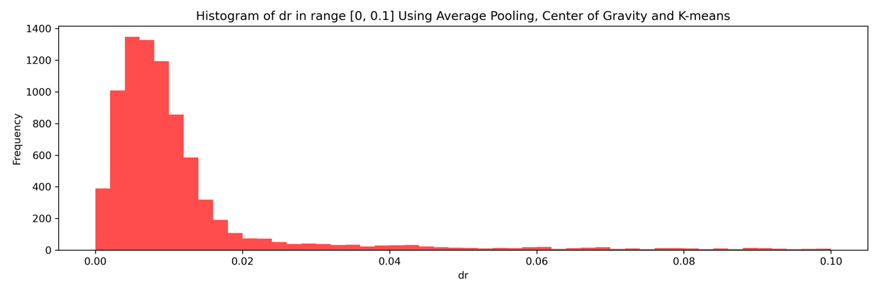
Figure 10. Histogram of dr in range [0, 0.1] using average pooling and k-Means

This method has several advantages over former ones. Compared to the method using local maximum and k-Means, it not only can predict more graphs with the right number of clusters, but also produces results with smaller standard deviation and smaller maximum of dr. At the same time, all the predicted centers are near real centers, so it resolves the problem that some predicted centers are actually not centers of clusters at all. Compared to the method that uses average pooling and center of gravity without k-Means, the standard deviation and the maximum of dr both become smaller, while the whole distribution shifts to the left. Meanwhile, it addresses the problem that the nearby centers will influence the prediction of position of centers. Thus, we can conclude that in our research, using average pooling, center of gravity and k-Means together is the best method to predict the center of clusters.

6. Result

6.1. Local Maximum & k-Means Approach

By using this method, we finally have 789 datasets successfully identify with 10 clusters. But the rest of them failed because the local maximum cannot accurately identify overlapping clusters’ mass center. They usually will be mistakenly recognized as single one mass center instead of two.

6.2. Convolutional Neural Network

This method is kind of a new approach, yet its results are not very good. The difference between validation loss and training loss is too large which leads to unstable outcome.

6.3. Average Pooling, Center of Gravity & k-Means

This approach is the most successful approach we have achieved. This method has identified 862 datasets with 10 clusters and precise mass center for both isolated clusters and overlapping clusters.

7. Conclusion

This study demonstrates that different methods possess their unique strengths and weaknesses in the cluster detection process.

The integration of Local Maximum and k-Means algorithms offers a powerful approach for identifying and optimizing the centers of mass within the dataset. The Local Maximum algorithm efficiently identifies potential centers with simple codes, while the k-Means algorithm ensures that the positions of centers can be predicted more accurately. This hybrid methodology exhibits precision for most of clusters. Our results, however, indicate that this method is not so effective under circumstances where clusters overlap, making it not suitable if high precision in image processing is required.

Convolutional Neural Networks is another method we employ. We make several attempts to let computer learn the images through deep learning, yet it does not yield very good effects. The positions of predicted centers do not match the positions of real centers. Maybe the computer is not learning in the way we expect.

The combination of Average Pooling with k-Means clustering emerges as a reliable strategy for predicting cluster centers in complex image datasets. This method capitalizes on the strengths of both algorithms to effectively address challenges such as overlapping clusters and noise interference, significantly improving the accuracy of cluster center identification.

This study provides a solid foundation for handling more challenging image processing tasks and offers valuable insights into the application of machine learning methods in cluster finding. To enhance the feasibility and accuracy of this approach to more diverse and intricate datasets, future work could explore further optimizations, including advanced clustering algorithms and additional data processing techniques.

Acknowledgement

We thank Prof. Gunther Roland of MIT for his guidance and advice on this study. Yiding Wang, Haoxi Xu and Shifan Hou contributed equally to this work and should be considered co-first authors. Yiding Wang have wrote the Abstract, some of part 1 Introduction, part 2 Local Maximum and k-Means, and part 6 Result, and responsible for all formatting issue. Haoxi Xu wrote part 4 Average Pooling & Center of Gravity, part 5 Average Pooling, Center of Gravity & k-Means, and part 7 Conclusion. Shifan Hou wrote part 3 Convolutional Neural Network. Shichen Wei is the second author who wrote some of part 1 Introduction.

References

[1]. Ran, X., Zhou, X., Lei, M., Tepsan, W., & Deng, W. (2021). A novel k-means clustering algorithm with a noise algorithm for capturing urban hotspots. Applied Sciences, 11(23), 11202.
[2]. Ikotun, A. M., Ezugwu, A. E., Abualigah, L., Abuhaija, B., & Heming, J. (2023). K-means clustering algorithms: A comprehensive review, variants analysis, and advances in the era of big data. Information Sciences, 622, 178-210.
[3]. Govender, P., & Sivakumar, V. (2020). Application of k-means and hierarchical clustering techniques for analysis of air pollution: A review (1980–2019). Atmospheric pollution research, 11(1), 40-56.
[4]. Yantovski-Barth, M., Newman, J. A., Dey, B., Andrews, B. H., Eracleous, M., Golden-Marx, J., & Zhou, R. (2024). The CluMPR galaxy cluster-finding algorithm and DESI legacy survey galaxy cluster catalogue. Monthly Notices of the Royal Astronomical Society, 531(2), 2285-2303.
[5]. Chen-xi, L. I., Bing, W. U., Fan, L. U. O., & Na, Z. H. A. N. G. (2020). Clinical study and CT findings of a familial cluster of pneumonia with coronavirus disease 2019 (COVID-19). JOURNAL OF SICHUAN UNIVERSITY (MEDICAL SCIENCES), 51(2), 155-158.
[6]. Li, Z., Liu, F., Yang, W., Peng, S., & Zhou, J. (2021). A Survey of Convolutional Neural Networks: Analysis, Applications, and Prospects. IEEE Transactions on Neural Networks and Learning Systems, 33(12), 1–21. https://doi.org/10.1109/tnnls.2021.3084827.
[7]. Chauhan, R., Ghanshala, K. K., & Joshi, R. C. (2018, December 1). Convolutional Neural Network (CNN) for Image Detection and Recognition. IEEE Xplore. https://doi.org/10.1109/ICSCCC.2018.8703316
[8]. Liu, S., & Deng, W. (2015, November 1). Very deep convolutional neural network based image classification using small training sample size. IEEE Xplore. https://doi.org/10.1109/ACPR.2015.7486599
[9]. Kandel, I., & Castelli, M. (2020). The effect of batch size on the generalizability of the convolutional neural networks on a histopathology dataset. ICT Express, 6(4). https://doi.org/10.1016/j.icte.2020.04.010
[10]. Bieder, F., Sandkühler, R., & Cattin, P. C. (2021). Comparison of Methods Generalizing Max- and Average-Pooling.
[11]. Kuhn, H. W. (1955). The Hungarian method for the assignment problem.
[12]. Gabrovšek, B., Novak, T., Povh, J., Poklukar, D. R., & Žerovnik, J. (2020). Multiple Hungarian Method for k-Assignment Problem. Mathematics.
Cite this article
Xu,H.;Wang,Y.;Hou,S.;Wei,S. (2025). Cluster Detection and Centers of Mass Prediction in Images. Applied and Computational Engineering,131,40-51.
Data availability
The datasets used and/or analyzed during the current study will be available from the authors upon reasonable request.
Disclaimer/Publisher's Note
The statements, opinions and data contained in all publications are solely those of the individual author(s) and contributor(s) and not of EWA Publishing and/or the editor(s). EWA Publishing and/or the editor(s) disclaim responsibility for any injury to people or property resulting from any ideas, methods, instructions or products referred to in the content.
About volume
Volume title: Proceedings of the 2nd International Conference on Machine Learning and Automation
© 2024 by the author(s). Licensee EWA Publishing, Oxford, UK. This article is an open access article distributed under the terms and
conditions of the Creative Commons Attribution (CC BY) license. Authors who
publish this series agree to the following terms:
1. Authors retain copyright and grant the series right of first publication with the work simultaneously licensed under a Creative Commons
Attribution License that allows others to share the work with an acknowledgment of the work's authorship and initial publication in this
series.
2. Authors are able to enter into separate, additional contractual arrangements for the non-exclusive distribution of the series's published
version of the work (e.g., post it to an institutional repository or publish it in a book), with an acknowledgment of its initial
publication in this series.
3. Authors are permitted and encouraged to post their work online (e.g., in institutional repositories or on their website) prior to and
during the submission process, as it can lead to productive exchanges, as well as earlier and greater citation of published work (See
Open access policy for details).