


1. Introduction
1.1. Background
In recent years, the global demand for rehabilitation services has grown explosively due to an ageing population, changing disease patterns and an increase in sports injuries. In order to meet the demand for rehabilitation therapy caused by the ageing population and the increase in the number of stroke patients, coupled with the insufficient number of rehabilitation therapists and the rising cost of manpower, rehabilitation robots, with their advantages of accuracy, high efficiency and controllability, have shown great potential in rehabilitation therapy [1,2,3]. The exoskeleton robot could be applied to alleviate the problems of an ageing population and insufficient healthcare resources while helping to reduce the burden on healthcare workers and lower the cost of treatment [2,3,4]. For further understanding, the technical direction could be generalized as three points: Spring Mechanism Integration, Simulation and Modeling, and Control System Optimization. The appearance of the rehabilitation robot is modeled after the structure of a human's lower extremities. Aside from the structure of traditional rehabilitation robots, a spring is added to the thigh and calve of the exoskeleton while a motor is installed on the knee [2]. The linear spring is used for gravity compensation in the new design of the exoskeleton while the motor is applied for energy provide [5]. The addition of the spring plays an essential role in preserving energy and balancing the body, enabling the user to move steadier and spend less energy on actions [1]. However, drawbacks still exist in the design.
1.2. Motivation
Based on the original commercially available rehabilitation robot, a lower limb rehabilitation robot is designed based on a spring assisted system [2]. This article is divided into four main parts: a brief introduction of the program, the proposed approach to achieve the goal, the results and conclusions of the project, and the plan for future work.
2. Proposed Approach
2.1. Baseline Hardware Set-up
2.1.1. MATLAB Simscape Building
When squatting, due to the symmetry of both legs, only the movement and force of one leg need to be considered. Therefore, the model established is a single leg robot, as shown in Figure 1. The lower long pole represents the lower leg of the exoskeleton, the upper long pole models the upper leg of the exoskeleton, and the cube on top of the long pole illustrates the load-bearing capacity, which indicates the external weight the exoskeleton can support [4]. Since the spring parameters between the legs are variables that require optimization, the spring is not directly added to the model; instead, an additional spring providing force is introduced during the simulation. The parameters of the exoskeleton, including angles and distances, are displayed in Figure 2. In order to conform to the movement laws of the lower limbs of the human body, the angle \( θ \) is set between -45 to 0 degrees. Table 1 outlines the key variables in the exoskeleton model, including the angle and angular velocity between the thigh and calf, as well as their expected values. It also defines the spring's original length, elastic coefficient, and the distance between the spring's ends and the knee. Additionally, the table explains the torques provided by the motor, muscles, and spring, as well as the horizontal and vertical forces acting on the calf. Important biomechanical factors such as muscle length, total torque, and energy consumption per cycle and over the simulation time are also covered, providing a complete overview of the system's dynamics. Table 2 presents the constant values used in the exoskeleton model. These include the lengths of the connecting rods representing both the thigh and calf, each measuring 0.4 meters, as well as the masses of both the thigh and calf, which are 15 kilograms each. These constants are essential for accurately simulating the mechanical behavior of the exoskeleton during movement. Based on the actual test rate, the following are the ranges of each variable:
\( 0.1m≤l≤0.4m \) (2.1)
\( 0.1m≤x≤0.3m \) (2.2)
\( 100N\cdot {m^{∧}}(-1)≤k≤1000N\cdot {m^{∧}}(-1) \) (2.3)

Figure 1. MATLAB Model.
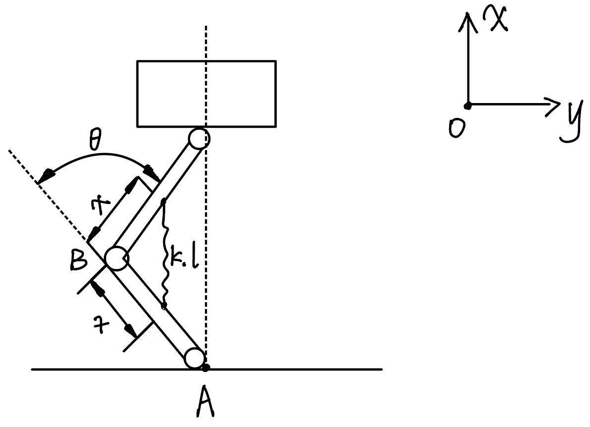
Figure 2. Exoskeleton parameters.
Table 1. Meaning of each variable.
Variable | Variable Meaning |
\( θ \) | The angle between the thigh and calf |
\( \dot{θ} \) | Angular velocity of thigh rotation |
\( {θ_{d}} \) | Expected angle between thigh and calf |
\( \dot{{θ_{d}}} \) | Expected value of thigh rotation angular velocity |
\( l \) | Original length of spring |
\( k \) | Elastic coefficient of spring |
\( x \) | The distance between the two ends of the spring and the knee |
\( {α_{1}} \) | Angular frequency |
\( {\dot{θ}_{{d_{max}}}} \) | Maximum thigh rotation angular velocity |
\( {τ_{motor}} \) | The torque provided by the motor |
\( {τ_{human}} \) | The torque provided by human muscles |
\( {τ_{spring}} \) | The torque provided by the spring |
\( {F_{s}} \) | The force provided by the spring |
\( {F_{1}} \) | The vertical force acting on the lower end of the calf |
\( {F_{2}} \) | The horizontal force acting on the lower end of the calf |
\( {F_{3}} \) | Load bearing is subjected to horizontal force |
\( {f_{muscle}} \) | The force exerted on human muscles |
\( {l_{muscle}} \) | Human muscle length |
\( {τ_{total}} \) | Total torque |
\( {E_{T}} \) | Energy consumption for one cycle |
\( E \) | Total energy consumption during simulation time |
Table 2. The value of a constant.
Variable | Value | Variable Meaning |
\( {l_{1}} \) | 0.4m | Length of connecting rod representing the thigh |
\( {l_{2}} \) | 0.4m | Length of connecting rod representing the calf |
\( {m_{1}} \) | 15kg | Mass of the thigh |
\( {m_{2}} \) | 15kg | Mass of the calf |
2.1.2. Kinematic Equations
To obtain various data of the exoskeleton during movement, it is necessary to plan a motion trajectory for it. In order to describe and calculate it concisely, conveniently, and in line with the behavior of the human lower limbs, it is assumed that the angle changes over time is [6].
\( {θ_{d}}=\frac{π}{4}sin({α_{1}}t)-\frac{π}{4} \) (2.4)
\( \dot{{θ_{d}}}=\frac{π}{4}{α_{1}}cos{(}{{α_{1}}t}) \) (2.5)
Considering that the speed of leg movement cannot be too fast or too slow, the following restrictions are required:
\( \dot{{θ_{d}}} \) ≤15(2.6)
According to 2.5,
\( {\dot{θ}_{{d_{max}}}}=\frac{π}{4}{α_{1}} \) (2.7)
so,
\( {α_{1}}≤\frac{60}{π} \) (2.8)
2.2. Simulation and control system
2.2.1. MATLAB Simulation
Figure 3 presents the detailed simulation model of the lower limb rehabilitation robot's control system, constructed within the MATLAB environment. This schematic diagram illustrates the interconnections between various components that are critical for the robot's operation. The model begins with the input variables \( θ \) (the angle between the thigh and calf) and \( \dot{θ} \) (the angular velocity of the thigh rotation). These variables are essential for calculating the desired joint angles and velocities. The controller block, marked with \( { K_{p}} \) and \( { K_{d}} \) , represents the proportional and derivative gains used in a PD (Proportional-Derivative) control scheme. These gains are crucial for determining the control input \( u \) that will adjust the motor torque to achieve the desired motion. The model also accounts for the torque provided by the motor, which are key in simulating the dynamic response of the exoskeleton.
These values are used in the feedback loop to compare with the actual joint states and compute the necessary control actions. The model culminates in the calculation of the total energy consumption, \( total\_energy \) , which is a critical parameter for evaluating the efficiency of the rehabilitation robot.
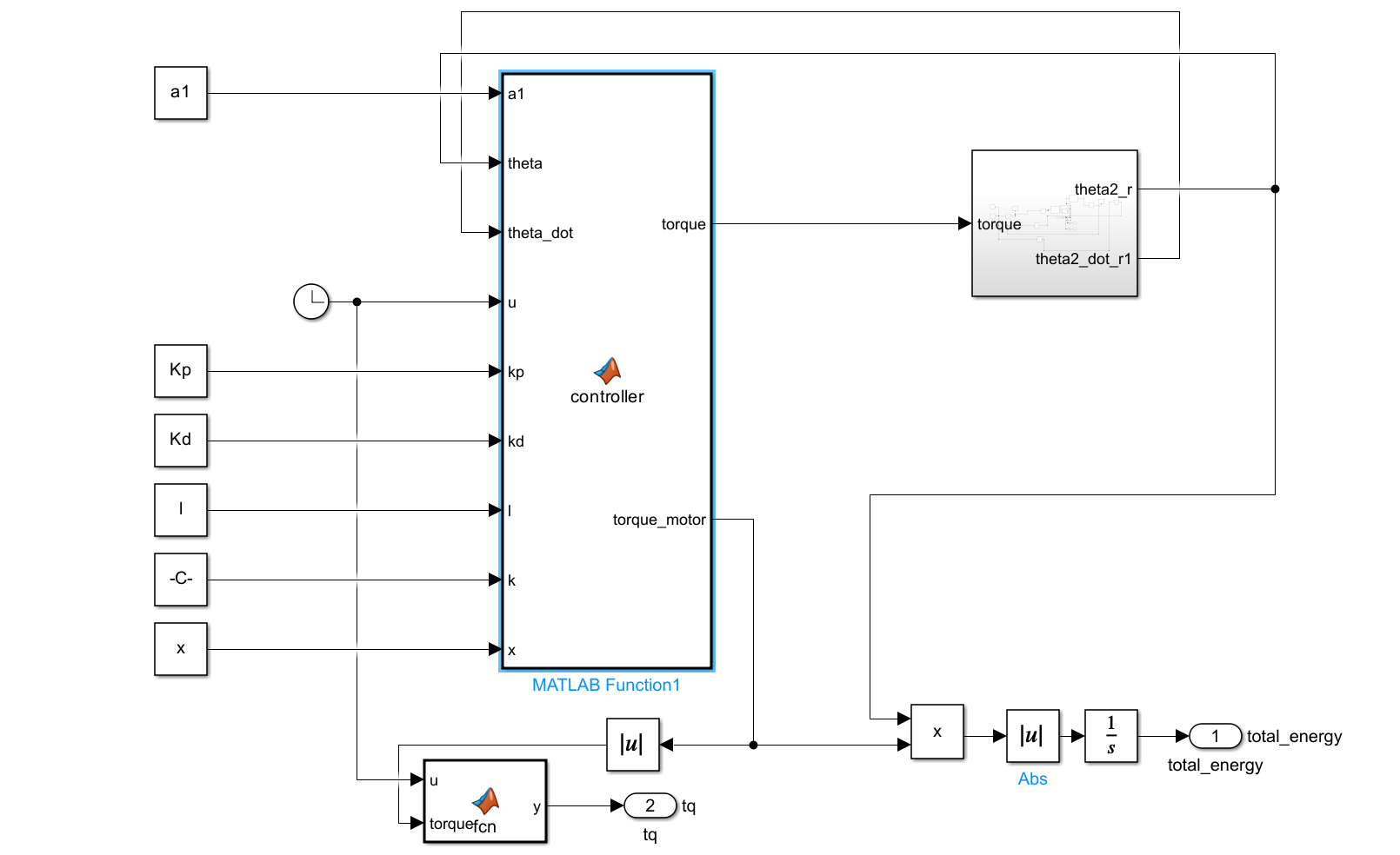
Figure 3. Simulation Model.
Figure 4 presents a detailed schematic of the subsystem model within the lower limb rehabilitation robot's overall control system. This subsystem is a critical component that interacts with the main system to ensure smooth and efficient operation. The model depicted in Figure 4 is designed to illustrate the configuration and interplay of various mechanical and control elements that contribute to the subsystem's functionality.
The subsystem is anchored by the “World Frame” and “Mechanism”, which serve as the foundational structure. The “Prismatic” joint and “Brick Solid1” and “Brick Solid2” are significant mechanical elements. The prismatic joint allows for linear motion, which is essential for simulating the translational movement in the robot's joints. “Brick Solid1” and “Brick Solid2” might represent different sections or components of the robot's structure that interact with each other to facilitate movement. Connections labeled as “Conn1” and “Conn2” are highlighted, indicating the flow of data or control signals between different parts of the subsystem. These variables are crucial for monitoring and controlling the motion of the robot's joints.
Figure 5 illustrates the structural layout of Subsystem1 and Subsystem2 within the lower limb rehabilitation robot. These subsystems are interconnected through labeled connection points “Conn1” and “Conn2”, ensuring seamless transfer of data and control signals throughout the system. The “Brick Solid” depicted in the diagram represents the key components of the robot's physical structure, playing a crucial role in providing stability and load-bearing capabilities [3].
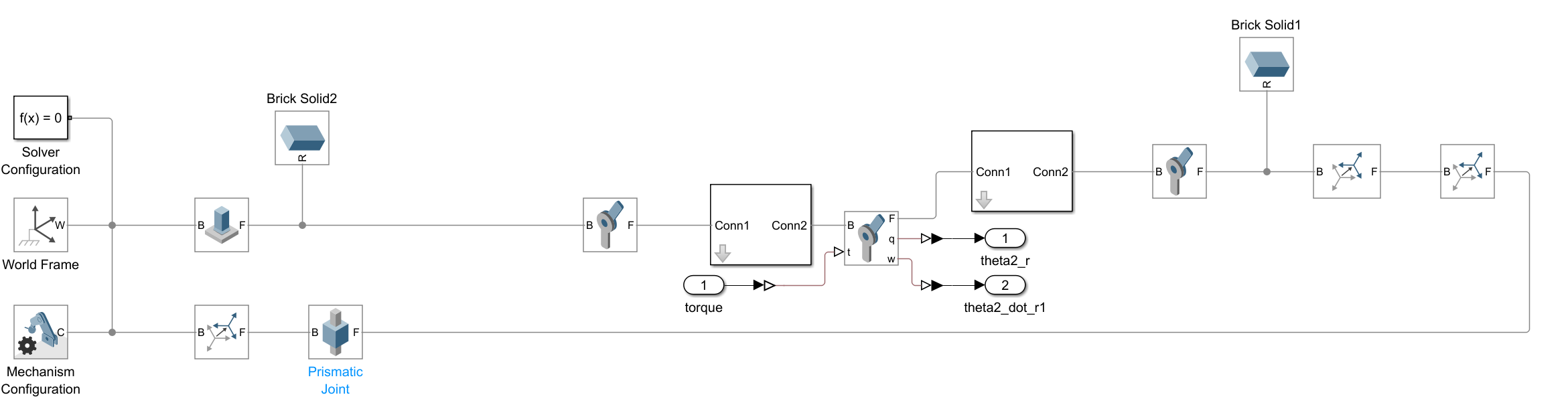
Figure 4. Model of Subsystem.
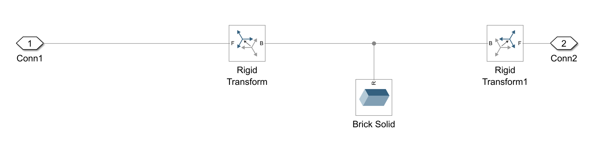
Figure 5. Model of Subsystem1 and Subsystem2.
2.2.2. Force Analysis
The force analysis is shown in the Figure 6. Because the research object is the exoskeleton at the knee and the research process is a squatting process, during which the human foot will be stationary due to the friction of the ground, the lower end of the calf can be fixed on the ground, and the lateral force \( {F_{2}} \) provided by the joint connection is equivalent to the frictional force. During squatting, a person can maintain balance in their upper body by exerting force on their abdomen, so the lateral force \( {F_{3}} \) provided by the M-axis is equivalent to the force used in the upper body of the human body. In addition to the torque provided by the motor in the exoskeleton and the torque provided by the spring, patients can provide a smaller amount of force based on the severity of lower limb paralysis [7].
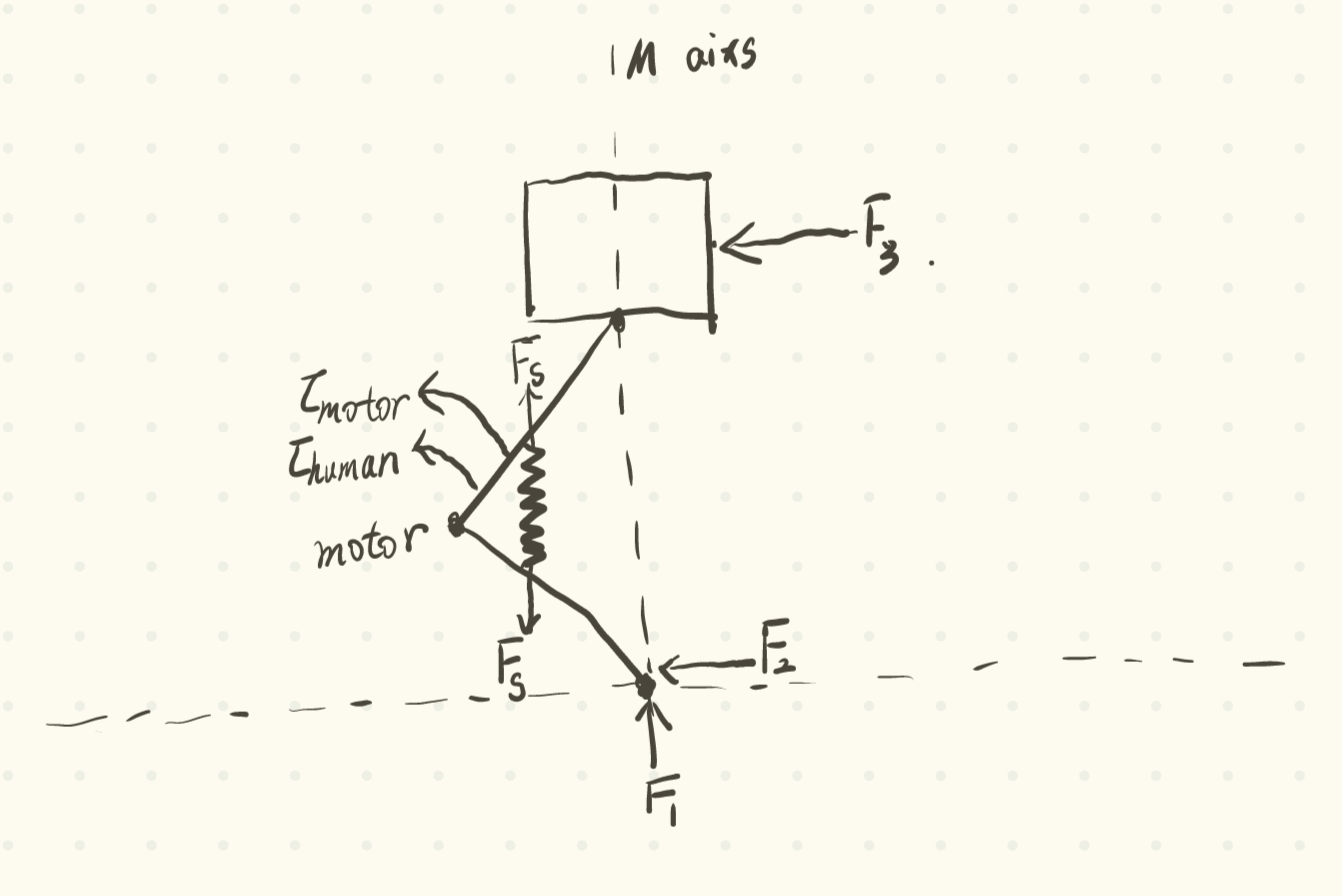
Figure 6. Force Analysis Diagram.
2.2.3. Joint control
The joint used to connect the calf to the ground is a revolute joint and the joints used in the knee is also a revolute joint. The calf can only rotate around point A in the plane XOY, and the thigh can only rotate around point B in the plane XOY (Figure 2). The joint between weight-bearing and thigh is a rotational joint while the joint between weight-bearing and M-axis is prismatic joint (Figure 6). The load can only move along the M-axis.
2.2.4. Controller
PD control is adopted for the control of exoskeleton movement, which means the torque provided by the motor is [8]
\( {τ_{motor}}={K_{p}}({θ_{d}}-θ)+{K_{d}}({\dot{θ}_{d}}-\dot{θ}) \) (2.9)
Due to the addition of springs in the design and the fact that human muscles can also provide torque, the torque input at the joints should also include the torque provided by the springs and the torque provided by the human. The force that leg muscles can provide varies with the severity of hemiplegia, and muscle length also varies from person to person. The provision of beneficial assistance in the real world is challenging for a number of reasons. Firstly, the sophisticated equipment utilized to personalize assistance is not readily accessible outside of laboratory settings. Secondly, in contrast to the controlled environment of a treadmill, everyday walking occurs in a multitude of bouts with varying speeds and durations. Thirdly, the devices must be self-contained and user-friendly. The values of muscle length and the force it provides are as follows
\( {f_{muscle}}=40N \) (2.10)
\( {l_{muscle}}=0.1m \) (2.11)
so the total torque input at the knee is
\( {τ_{total}}={τ_{motor}}+{τ_{spring}}+{τ_{human}} \) (2.12)
where
\( {τ_{spring}}={f_{spring}}xsin(-\frac{θ}{2}) \) (2.13)
\( {τ_{human}}={f_{muscle}}{l_{muscle}}sin(\frac{-θ}{2}) \) (2.14)
\( {f_{spring}}=k(l-2xsin(\frac{θ+π}{2})) \) (2.15)
2.3. Energy consumption set-up
2.3.1. Optimization
The formula for the energy consumed by the exoskeleton is [9]
\( {E_{T}}=\frac{2πE}{{α_{1}}{t_{f}}} \) (2.16)
\( E=\int _{0}^{{t_{f}}}{τ_{motor}}\dot{θ}dt \) (2.17)
And according to the actual situation, a motor on the exoskeleton can provide a maximum torque of approximately 50 N·m, because an exoskeleton has two motors so
\( {τ_{motor}}≤100N\cdot m \) (2.18)
The energy consumption of an exoskeleton in one cycle needs to be simulated to obtain its value, which is related to the following parameters:
\( l,k,x,{K_{p}},{K_{d}},{α_{1}} \)
Due to the large number of variables and the inability to find an exact functional relationship between the variables and the target, genetic algorithm can be used to optimize.
2.3.2. Results
Table 3 displays the outcomes of genetic algorithm optimization for the lower limb rehabilitation robot, detailing how key parameters adjust under varying load conditions to enhance the robot's energy efficiency. The table lists the optimized values for each load, demonstrating the robot's adaptability and the effectiveness of the optimization in reducing energy consumption per cycle[10].
As shown in Table 3, the optimization process fine-tunes parameters such as control gains, mechanical dimensions, and spring constants to achieve better performance across a range of loads.
Table 3. Optimized values of various parameters.
\( m \) (kg) | \( {K_{p}} \) | \( {K_{d}} \) | \( l \) (m) | \( k \) (N/m) | \( x \) (m) | \( {α_{1}} \) | Energy consumption for each cycle |
5 | 935.467270 | 297.075469 | 0.392916 | 971.256979 | 0.125047 | 6.491127 | 23.020137 |
10 | 961.756152 | 318.522157 | 0.393604 | 949.760362 | 0.119346 | 7.120287 | 35.241748 |
15 | 996.804930 | 638.641146 | 0.379914 | 985.885957 | 0.114353 | 5.249863 | 52.213038 |
20 | 965.105404 | 406.920326 | 0.391537 | 995.288970 | 0.116241 | 4.369228 | 71.713899 |
25 | 974.216383 | 623.052734 | 0.374290 | 977.922104 | 0.121310 | 2.756499 | 128.174321 |
27 | 965.490651 | 542.331337 | 0.387635 | 958.815479 | 0.130557 | 2.593458 | 141.403584 |
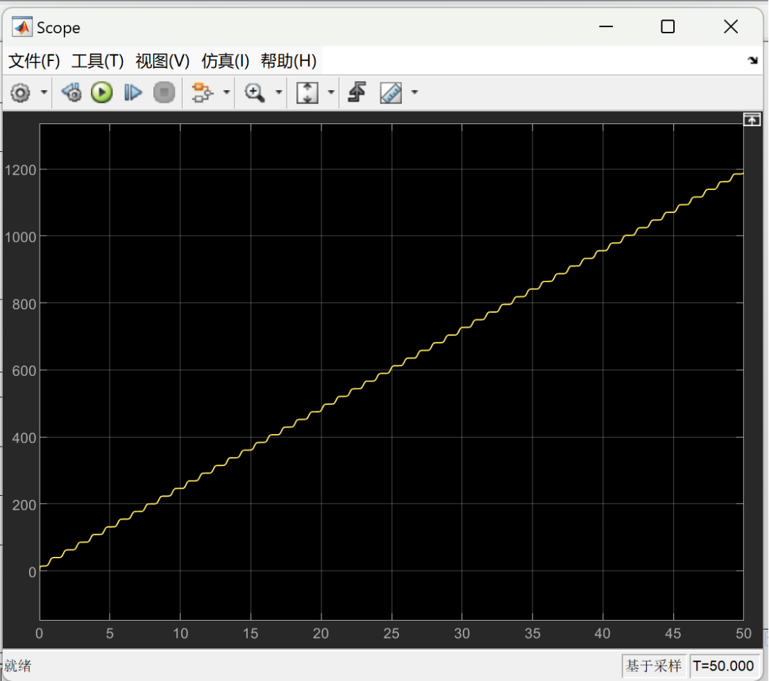
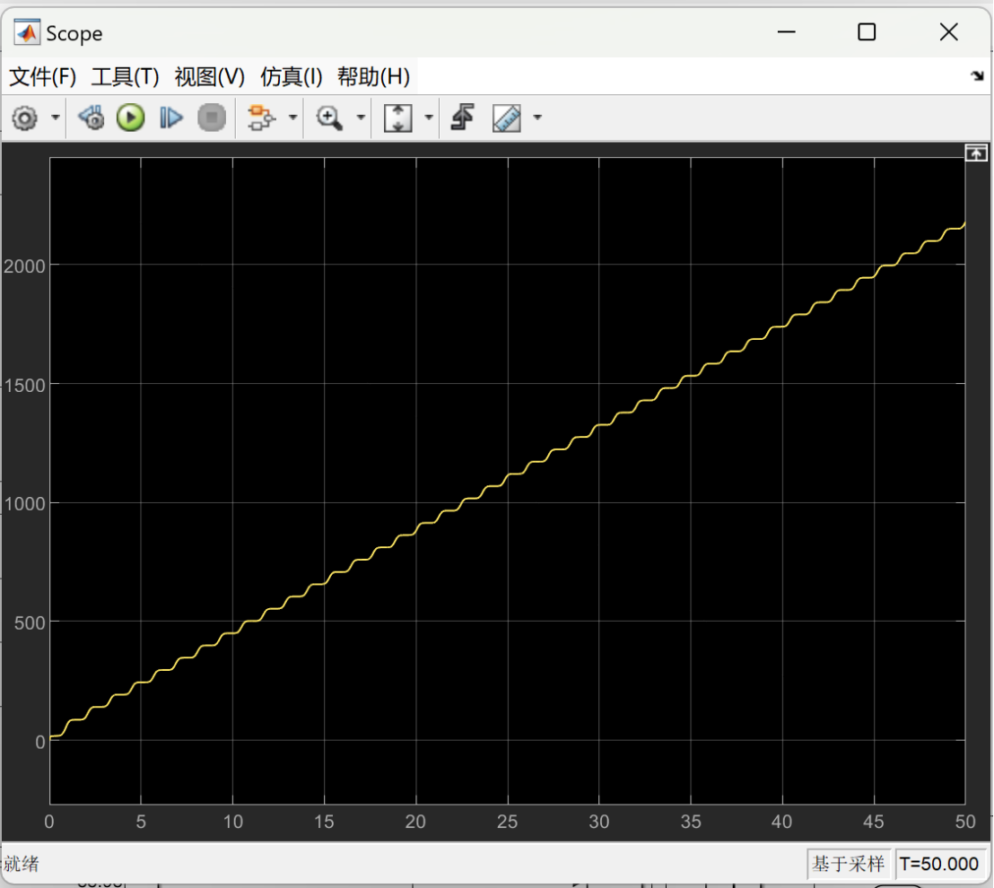
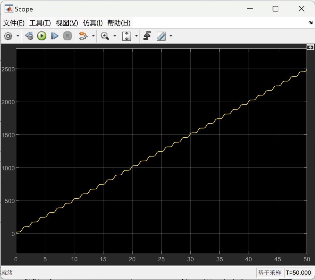
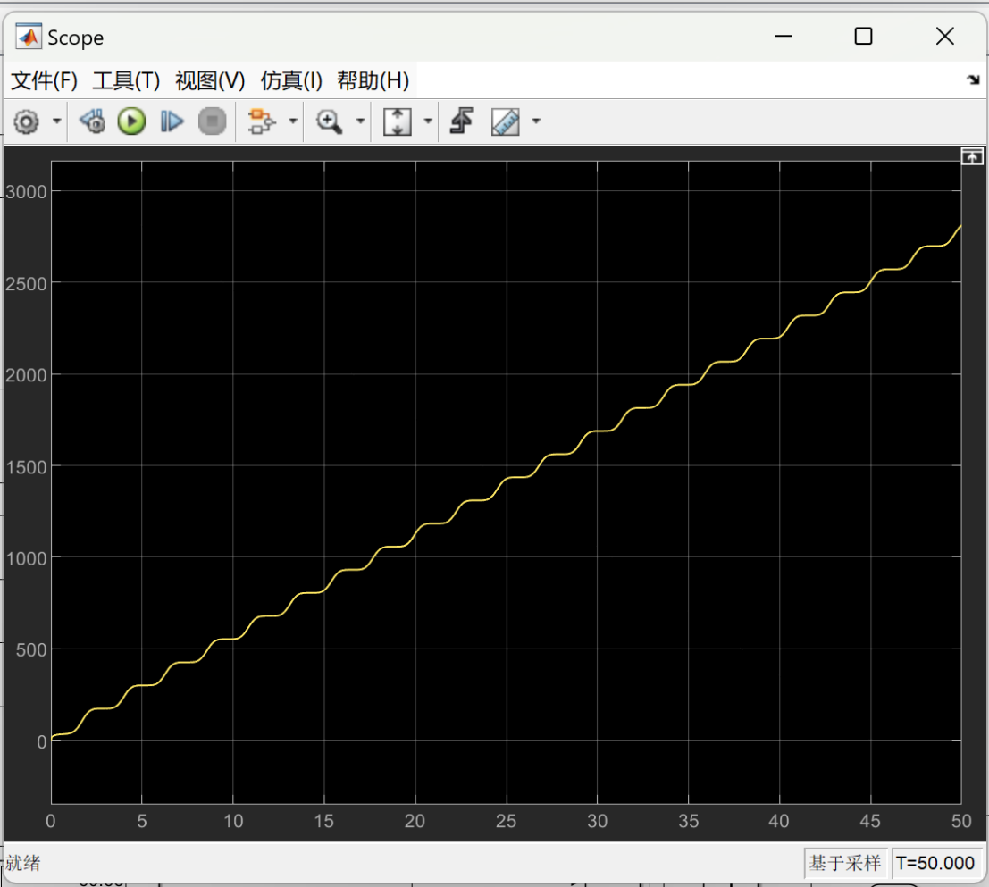
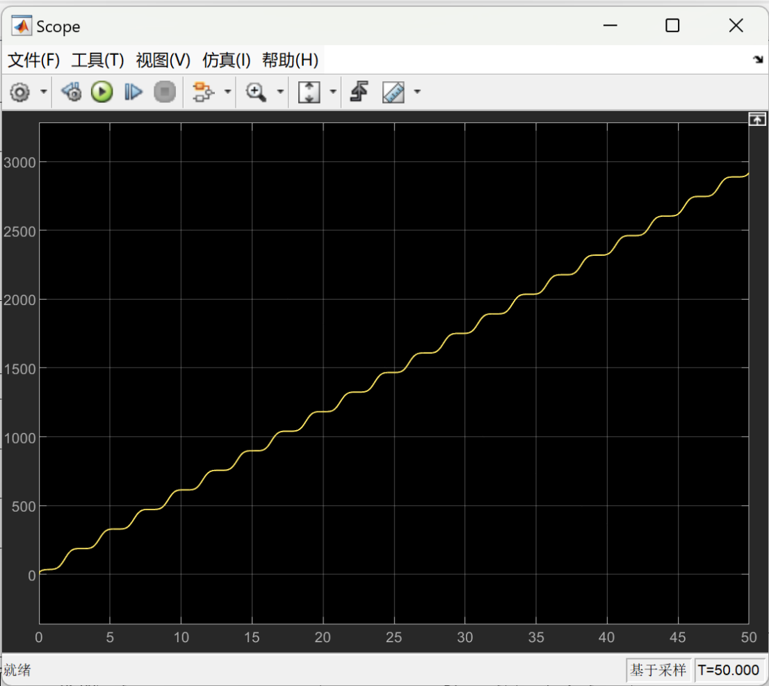
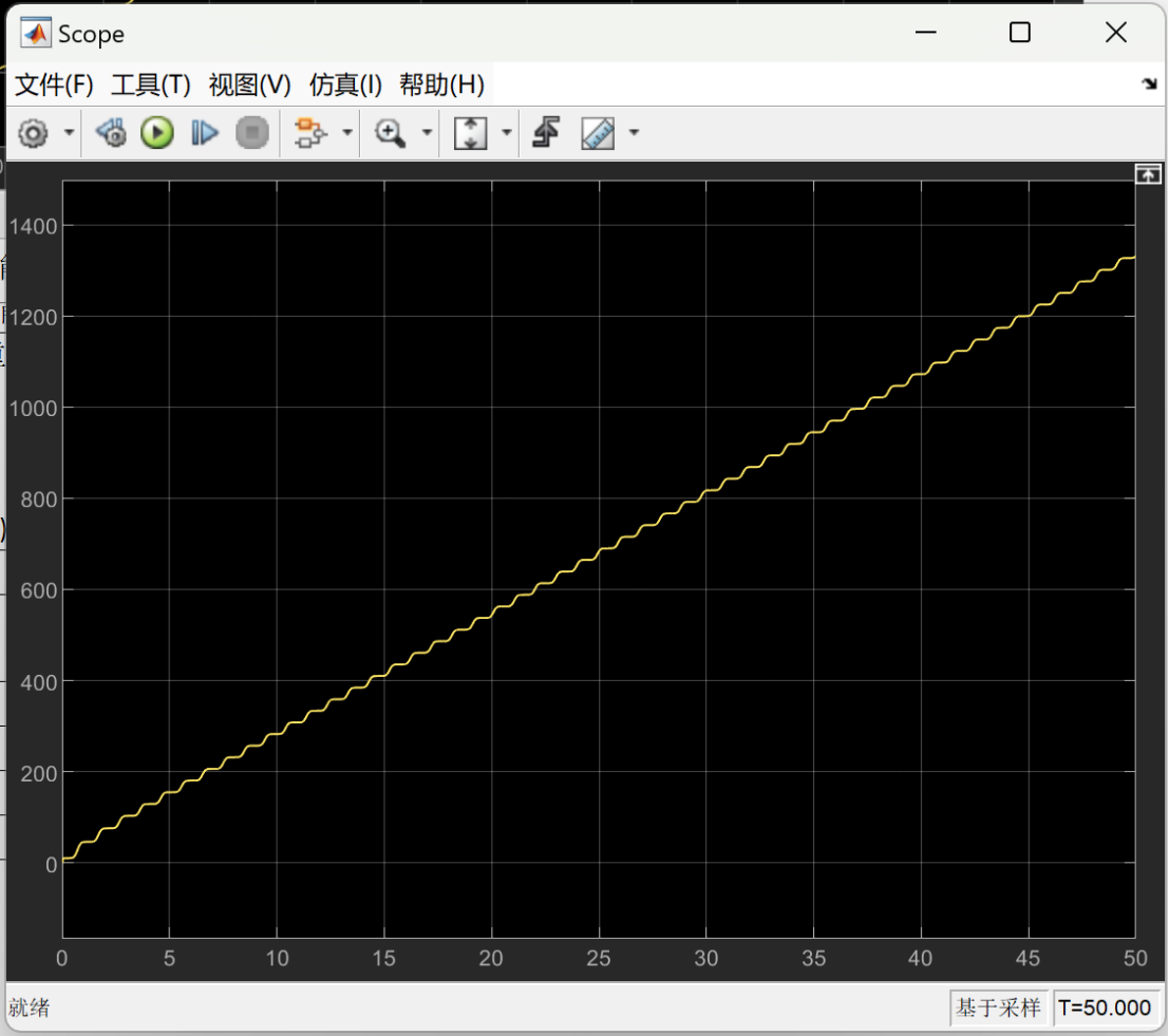
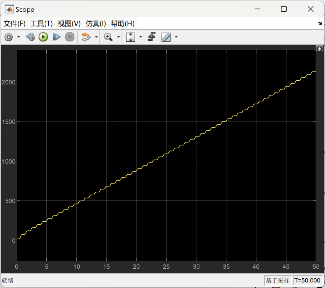
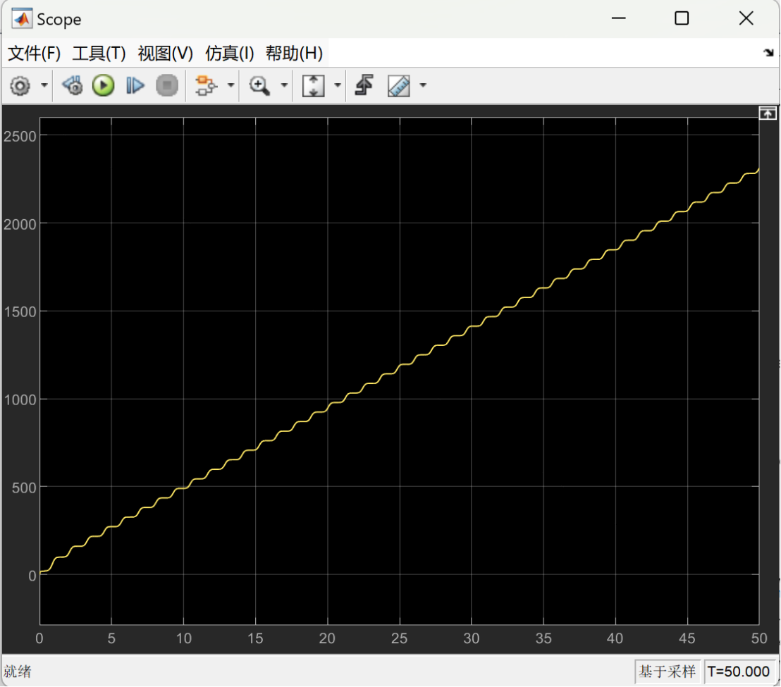
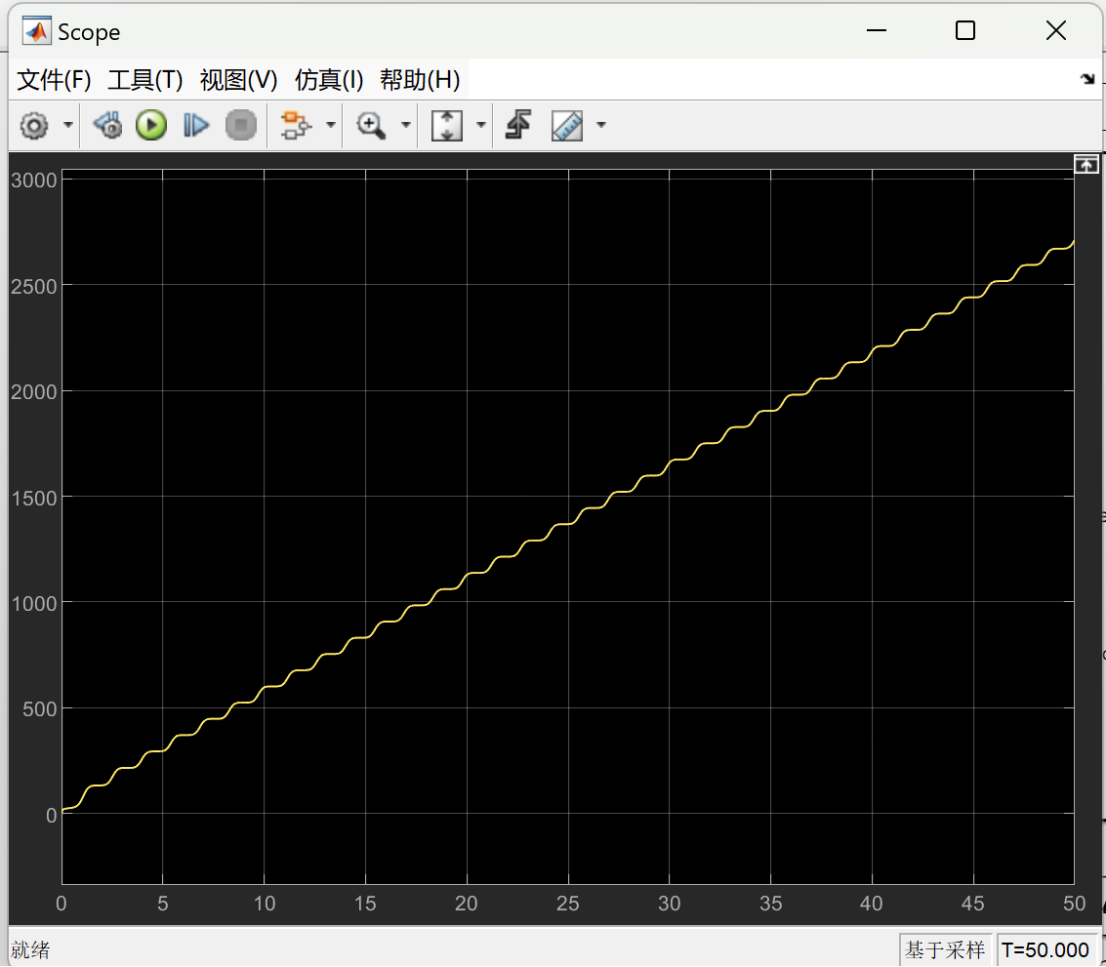
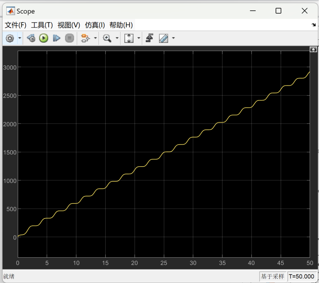
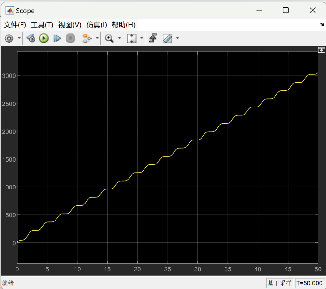
The following images show the optimized energy consumption curve over time under different load weights. The X-axis represents time, which shows the energy consumption of the lower limb rehabilitation robot at different time points. The Y-axis represents the measure of energy consumption, indicating the optimized energy consumption of the robot over time.
Figure 7 depicts the optimized energy consumption curve for the lower limb rehabilitation robot when the load is set at 5 kg. Figure 8 presents the optimized energy consumption curve for the lower limb rehabilitation robot when the load is 10 kg. Figure 9 presents the optimized energy consumption curve for the robot when subjected to a 15 kg load. Figure 10 displays the energy consumption curve optimized for a 20 kg load. Figure 11 shows the optimized energy consumption curve when the load is increased to 25 kg. Figure 12 illustrates the optimized energy consumption curve for the highest load tested, 27 kg. The graph is instrumental in showing the robot's energy efficiency at the upper limit of its load-bearing capacity, crucial for ensuring the robot's reliability and effectiveness in practical rehabilitation applications. Energy consumption generally increases as the load increases. This is because the robot requires more energy to overcome the greater gravity and drag. The optimized energy consumption curve shows the robot's improved energy efficiency at different loads. This shows that the robot's performance can be improved by optimizing the control algorithm and mechanical design.
|
|
Figure 7. When the load is 5 kg, the optimized energy consumption curve over time. | Figure 8. When the load is 10 kg, the optimized energy consumption curve over time. |
|
|
Figure 9. When the load is 15 kg, the optimized energy consumption curve over time. | Figure 10. When the load is 20 kg, the optimized energy consumption curve over time. |
|
|
Figure 11. When the load is 25 kg, the optimized energy consumption curve over time. | Figure 12. When the load is 27 kg, the optimized energy consumption curve over time. |

For the convenience of comparison, the periods before and after optimization were made the same, and the values of other variables were changed to compare the energy consumption of the two. Table 4 presents the values of each parameter prior to optimization.
Table 4. The values of each parameter before optimization.
\( m \) (kg) | \( {K_{p}} \) | \( {K_{d}} \) | \( l \) (m) | \( k \) (N/m) | \( x \) (m) | \( {α_{1}} \) | Energy consumption for each cycle |
5 | 1000 | 1000 | 0.4 | 1000 | 0.2 | 6.491127 | 25.786594 |
10 | 1000 | 1000 | 0.4 | 1000 | 0.2 | 7.120287 | 37.679944 |
15 | 1000 | 1000 | 0.4 | 1000 | 0.2 | 5.249863 | 55.389220 |
20 | 1000 | 1000 | 0.4 | 1000 | 0.2 | 4.369228 | 78.000043 |
25 | 1000 | 1000 | 0.4 | 1000 | 0.2 | 2.756499 | 133.117415 |
27 | 1000 | 1000 | 0.4 | 1000 | 0.2 | 2.593458 | 147.881952 |
The following images show the energy consumption curve over time before optimization under different load weights.
Figure 13 displays the energy consumption curve for the lower limb rehabilitation robot under a 5 kg load, before optimization. The graph tracks energy usage over time, offering a baseline to compare the efficiency improvements achieved through genetic algorithm optimization. Figure 14 presents the energy consumption curve for the lower limb rehabilitation robot when the load is 10 kg, before any optimization measures were applied. The graph tracks the robot's energy usage over a 50-unit time period, starting from the initial 5 units. This data serves as a reference point to evaluate the impact of optimization on the robot's energy efficiency. Figure 15 illustrates the energy consumption curve of the lower limb rehabilitation robot under a 15 kg load, before optimization. Figure 16 depicts the energy consumption curve for the lower limb rehabilitation robot under a 20 kg load, before optimization. Figure 17 illustrates the energy consumption curve for the robot under a 25 kg load, also before optimization. Figure 18 presents the energy consumption curve for the robot under the highest load considered, 27 kg, before any optimization.
|
|
Figure 13. When the load is 5 kg, energy consumption curve over time before optimization. | Figure 14. When the load is 10 kg, energy consumption curve over time before optimization. |
|
|
Figure 15. When the load is 15 kg, energy consumption curve over time before optimization. | Figure 16. When the load is 20 kg, energy consumption curve over time before optimization. |
|
|
Figure 17. When the load is 25 kg, energy consumption curve over time before optimization. | Figure 18. When the load is 27 kg, energy consumption curve over time before optimization. |
To facilitate a more intuitive comparison of energy consumption before and after optimization, Table 5 has been designed to present the values side by side. This arrangement allows for a direct visual assessment of the impact of the optimization process on the energy efficiency of the lower limb rehabilitation robot under various load conditions. As demonstrated in Table 5, the optimized energy consumption for each cycle is notably reduced compared to the values recorded prior to optimization, indicating the effectiveness of the implemented improvements.
Table 5. Comparison of energy consumption before and after optimization.
m (kg) | Energy consumption per cycle before optimization | Optimized energy consumption for each cycle |
5 | 25.786594 | 23.020137 |
10 | 37.679944 | 35.241748 |
15 | 55.389220 | 52.213038 |
20 | 78.000043 | 71.713899 |
25 | 133.117415 | 128.174321 |
27 | 147.881952 | 141.403584 |
3. Discussion
The designed model can achieve both sitting to standing and standing to sitting, and energy consumption can be reduced to some extent through genetic algorithm optimization. However, in the case where each motor provides a torque of less than 50 N/m, it cannot support a load greater than 27 kg. However, the mass of the upper body of the human body is often much greater than 27 kg, and the maximum torque limit of each motor can be increased to solve this problem.
Aside from that, the financial considerations are also crucial. Increasing the motor's torque capacity may involve higher costs for more powerful motors and potentially more complex control systems to manage the additional torque. However, this investment could be offset by the benefits of a robot that can support a wider range of patients and provide more versatile assistance in rehabilitation settings. It is also important to consider the cost of energy savings over time, as the optimized model's reduced energy consumption could lead to significant savings in the long run, which could justify the initial increased investment.
Moreover, the optimization not only affects the mechanical and financial aspects but also has implications for patient comfort and therapy outcomes. A robot that can handle more significant loads with less energy consumption is likely to provide smoother and more natural assistance, which could lead to better compliance with therapy regimens and improved rehabilitation outcomes.
In conclusion, while the current model demonstrates promising results in terms of energy efficiency and functionality, there is room for further enhancement. Future work should focus on motor upgrades, control system refinements, and economic analyses to ensure that the robot meets both the practical needs of users and the financial constraints of healthcare providers. This comprehensive approach will be vital in realizing the full potential of the rehabilitation robot and its impact on patient care.
4. Conclusion
The lower limb rehabilitation robot with a spring-assisted system shows great potential for future rehabilitation therapy [10]. The integration of a spring mechanism and optimization using a genetic algorithm successfully reduced motor energy consumption, enhancing efficiency and practicality for daily use. The robot's adaptability to different user needs, tested through load capacity optimization, is a key achievement. However, further improvements are needed, particularly in motion control precision and increasing the maximum load capacity [11]. Future work should focus on refining these areas and integrating advanced sensors for more adaptive control systems. While significant progress has been made, continued innovation is essential to fully realize the potential of this technology in meeting global rehabilitation demands.
Acknowledgement
Sixuan Wu, Ruoshan Huang, Haotong Jiang contributed equally to this work and should be considered co-first authors.
References
[1]. Zhou, L., Chen, W., Chen, W., Bai, S., Zhang, J., Wang, J. (2020). Design of a passive lower limb exoskeleton for walking assistance with gravity compensation. (Mechanism and Machine Theory), pp.150-152.
[2]. Chen, W., Lyu, M., Ding, X., Wang, J., Zhang, J. (2024). Electromyography-controlled lower extremity exoskeleton to provide wearers flexibility in walking. (Mechanism and Machine Theory), pp.150-152.
[3]. Lakmazaheri, A., Song, S., Vuong, B.B., Biskner, B., Kado, D.M., Collins, S.H. (2024). Optimizing exoskeleton assistance to improve walking speed and energy economy for older adults. (Journal of NeuroEngineering and Rehabilitation), p21.
[4]. Slade, P., Kochenderfer, M.J., Delp, S.L., Collins, S.H. (2022). Personalizing exoskeleton assistance while walking in the real world. (Nature), pp.277-282.
[5]. Scott, E. (2019). The anxious leg bounce: Why it happens and how to deal with it. https://metro.co.uk/2019/04/20/anxious-leg-bounce-happens-deal-9277508/
[6]. Anon. (no date). Amplitude, period, phase shift and frequency. https://www.mathsisfun.com/algebra/amplitude-period-frequency-phase-shift.html
[7]. Cieza, A., Causey, K., Kamenov, K., Hanson, S.W., Chatterji, S., Vos, T. (2020). Global estimates of the need for rehabilitation based on the global burden of disease study 2019: A systematic analysis. (THE LANCET), pp.2006-2017.
[8]. Google Classroom. (nd). Torque. https://www.googleclassroom.com/torque.
[9]. Khan Academy. (no date). Conservation of energy review. https://www.khanacademy.org/conservation-of-energy.
[10]. Jorgenson, K.W., Phillips, S.M., Hornberger, T.A. (2024). Identifying the structural adaptations that drive the mechanical load-induced growth of skeletal muscle: A scoping review. https://www.ncbi.nlm.nih.gov/pmc/articles/PMC7408414/
[11]. Lung, C.W., Liau, B.Y., Peters, J.A., He, L., Townsend, R., Jan, Y.K. (2021). Effects of various walking intensities on leg muscle fatigue and plantar pressure distributions. (National Library of Medicine), pp.22-27.
Cite this article
Wu,S.;Huang,R.;Jiang,H.;Wan,J. (2025). Optimize the Design of a Lower Limb Rehabilitation Robot Based on a Spring Assisted System. Applied and Computational Engineering,132,119-130.
Data availability
The datasets used and/or analyzed during the current study will be available from the authors upon reasonable request.
Disclaimer/Publisher's Note
The statements, opinions and data contained in all publications are solely those of the individual author(s) and contributor(s) and not of EWA Publishing and/or the editor(s). EWA Publishing and/or the editor(s) disclaim responsibility for any injury to people or property resulting from any ideas, methods, instructions or products referred to in the content.
About volume
Volume title: Proceedings of the 2nd International Conference on Machine Learning and Automation
© 2024 by the author(s). Licensee EWA Publishing, Oxford, UK. This article is an open access article distributed under the terms and
conditions of the Creative Commons Attribution (CC BY) license. Authors who
publish this series agree to the following terms:
1. Authors retain copyright and grant the series right of first publication with the work simultaneously licensed under a Creative Commons
Attribution License that allows others to share the work with an acknowledgment of the work's authorship and initial publication in this
series.
2. Authors are able to enter into separate, additional contractual arrangements for the non-exclusive distribution of the series's published
version of the work (e.g., post it to an institutional repository or publish it in a book), with an acknowledgment of its initial
publication in this series.
3. Authors are permitted and encouraged to post their work online (e.g., in institutional repositories or on their website) prior to and
during the submission process, as it can lead to productive exchanges, as well as earlier and greater citation of published work (See
Open access policy for details).
References
[1]. Zhou, L., Chen, W., Chen, W., Bai, S., Zhang, J., Wang, J. (2020). Design of a passive lower limb exoskeleton for walking assistance with gravity compensation. (Mechanism and Machine Theory), pp.150-152.
[2]. Chen, W., Lyu, M., Ding, X., Wang, J., Zhang, J. (2024). Electromyography-controlled lower extremity exoskeleton to provide wearers flexibility in walking. (Mechanism and Machine Theory), pp.150-152.
[3]. Lakmazaheri, A., Song, S., Vuong, B.B., Biskner, B., Kado, D.M., Collins, S.H. (2024). Optimizing exoskeleton assistance to improve walking speed and energy economy for older adults. (Journal of NeuroEngineering and Rehabilitation), p21.
[4]. Slade, P., Kochenderfer, M.J., Delp, S.L., Collins, S.H. (2022). Personalizing exoskeleton assistance while walking in the real world. (Nature), pp.277-282.
[5]. Scott, E. (2019). The anxious leg bounce: Why it happens and how to deal with it. https://metro.co.uk/2019/04/20/anxious-leg-bounce-happens-deal-9277508/
[6]. Anon. (no date). Amplitude, period, phase shift and frequency. https://www.mathsisfun.com/algebra/amplitude-period-frequency-phase-shift.html
[7]. Cieza, A., Causey, K., Kamenov, K., Hanson, S.W., Chatterji, S., Vos, T. (2020). Global estimates of the need for rehabilitation based on the global burden of disease study 2019: A systematic analysis. (THE LANCET), pp.2006-2017.
[8]. Google Classroom. (nd). Torque. https://www.googleclassroom.com/torque.
[9]. Khan Academy. (no date). Conservation of energy review. https://www.khanacademy.org/conservation-of-energy.
[10]. Jorgenson, K.W., Phillips, S.M., Hornberger, T.A. (2024). Identifying the structural adaptations that drive the mechanical load-induced growth of skeletal muscle: A scoping review. https://www.ncbi.nlm.nih.gov/pmc/articles/PMC7408414/
[11]. Lung, C.W., Liau, B.Y., Peters, J.A., He, L., Townsend, R., Jan, Y.K. (2021). Effects of various walking intensities on leg muscle fatigue and plantar pressure distributions. (National Library of Medicine), pp.22-27.