1. Introduction

Spill-free transportation of liquids has a wide range of applications across industries where liquid products need to be transported efficiently, safely, and with minimal loss or environmental impact. These applications include (1) handling of beverage or liquid food, (2) handling of sterile liquids or biological samples in the pharmaceutical and biotechnology industry, (3) handling of hazardous or corrosive chemicals. pesticides or wastewater, (4) handling of oil or liquefied natural gas, (5) handling of other types of liquid such as perfumes, and coolants, and (6) bulk liquid transportation or intermediate bulk containers and tankers.

The advantages in using autonomous robots to transport or move open-top liquid containers are mainly safety, accuracy, scalability and predictability.

Previously, spill-free robotic model relied heavily upon the understanding of the physics of fluid dynamics, computational fluid dynamics, and related modifications. Due to the complexity involved in fluid dynamics, small particles were used to represent the fluid as an approximation. However, a fluid control mechanism is still challenging to develop. Thus, previous approaches have been focused on smoothing the motion to minimize jerks and accelerations, or tilting the container to compensate the spill dynamics.

The invention of the SpillNot device is a breakthrough in fluid control mechanisms. Instead of analyzing fluid dynamics at a miniscule level, it aggregates everything at the end effector, including the gripper, the container and the liquid as one mass under the pendulum model. Under the pendulum motion equation, as long as this mass moves along the pendulum trajectory, all parts of the mass stay together, hence no spills.

To take one step further, by simulating and controlling the pendulum motion, a robotic arm can move liquid spill-free along the spill-free trajectories, replacing the SpillNot device. Furthermore, the feedback control mechanism of the autonomous robot results in accurate real-time spill-free fluid maneuvers and transportation.

Thus, a PID-controlled Simulink and Simscape model will help further demonstrate the application of the pendulum model in autonomous robots to achieve spill-free liquid transportation and provide a working model for further development of the stability of robotics handling various kinds of liquid in various settings as described at the beginning of this introduction.

2. Mathematical Model

2.1. Simple Pendulum Equation

A pendulum is a body suspended from a fixed support such that it freely swings back and forth under the influence of gravity. A simple gravity pendulum is an idealized mathematical model of a real pendulum. It is a weight (or bob) on the end of a massless cord suspended from a pivot, without friction.

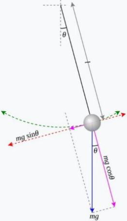
Figure 1. Simple pendulum

where g is the magnitude of the gravitational field, ℓ is the length of the rod or cord, and θ is the angle from the vertical to the pendulum.

Note that the path of the pendulum sweeps out an arc of a circle. The angle θ is measured in radians, and this is crucial for this formula. The blue arrow is the gravitational force acting on the bob, and the violet arrows are that same force resolved into components parallel and perpendicular to the bob's instantaneous motion. The direction of the bob's instantaneous velocity always points along the red axis, which is considered the tangential axis because its direction is always tangent to the circle. Consider Newton's second law, F=ma.

Newton's equation can be applied to the tangential axis only. This is because only changes in speed are of concern and the bob is forced to stay in a circular path. The short violet arrow represents the component of the gravitational force in the tangential axis, and trigonometry can be used to determine its magnitude. Thus,

where g is the acceleration due to gravity near the surface of the earth. The negative sign on the right-hand side implies that θ and α always point in opposite directions. This makes sense because when a pendulum swings further to the left, it is expected to accelerate back toward the right.

This linear acceleration a along the red axis can be related to the change in angle θ by the arc length formulas; s is arc length:

thus:

2.2. Spherical Pendulum Model

The spherical pendulum model is also called 3D pendulum model. When the pendulum swings, there are no lateral reaction forces nor external torques acting on the container. Total reaction force is aligned with the pendulum’s vertical direction and its line of action passes through the object’s center of mass. The relationship between the lateral acceleration α_x, vertical acceleration α _z, the gravity acceleration g and the tilt angle θ is therefore given by (α_z + g) tan θ = α_x. The parametrization is based on the linear model of the pendulum.

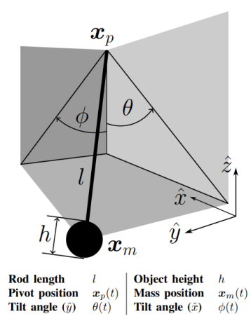
Figure 2. Spherical pendulum

2.3. Euler-Lagrange Equations of Motion

The Euler-Lagrange equations is a widely used fluid dynamic equation for the motion in the spherical pendulum model, in which, the rod the length l is taken as weightless and no friction sources affect the motion. The position of the mass follows below equation:

The mass of the system is concentrated at this point and the total energy is therefore determined by the motion therein—the evolution of x_m with time. The kinetic energy K and potential energy U of the system can be calculated as

Building the Lagrangian L := K − U and applying the Euler-Lagrange equation gives the equations of motion of the system,

The pendulum motion allows the system to achieve slosh-free condition. [3]

3. Matlab Design and Approach

The challenge of this project is to keep the liquid stable during the robot’s motion. This involves precise control of the end-effector's angles to ensure that the container remains upright while the 3-DOF robotic arm moves along a predefined trajectory. Simscape models the physical behavior and kinematics of the robotic system, while Simulink simulates the feedback and control required for stability.

3.1. Kinematic Modeling in Simscape

In the Simscape environment, the 5-DOF robotic system is broken down into its kinematic components. [4] The 3-DOF robot arm is responsible for moving the end-effector along the trajectory in 3D space (controlling the position in x, y, and z coordinates). The end-effector, attached at the arm’s tip, provides two additional degrees of freedom, enabling the adjustment of the container’s tilt and rotation.

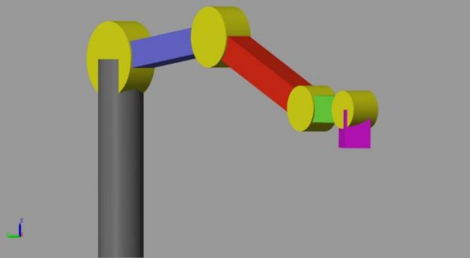
Figure 3. Front view of the 5-DOF robotic system in Simscape (end-effector is shown in bright pink at the arm’s tip)

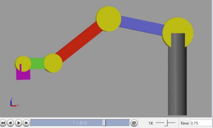
Figure 4. Side view of the 5-DOF robotic system in Simscape

Simscape models the physical dynamics of the robot based on the Denavit-Hartenberg (D-H) parameters, which define the relative transformations between the robot's links and joints. In this kinematic simulation, the arm follows the input trajectory, and the movement is accurately reflected by Simscape’s physics engine. However, in this model, only the robot's motion and the relative positions of its links are simulated; the orientation of the container, while kinematically determined, is not automatically balanced to prevent liquid spillage.

This is where the 2-DOF end-effector comes into play. [5] As the arm moves along the defined path, the end-effector's two joints need to be adjusted continuously to keep the container aligned with the global z-axis, preventing the liquid from tilting. Simscape provides the kinematic calculations needed to model the motion, but the balancing of the liquid requires a control system that is implemented in Simulink.

3.2. Simulink PID Control for End-Effector Orientation

While Simscape handles the robot’s kinematics, the actual control of the end-effector’s orientation to maintain the liquid’s stability is achieved in Simulink using a PID controller. [6] The end-effector has two degrees of freedom, responsible for controlling the tilt and rotation of the container. The PID controller ensures that the container remains upright, regardless of the robot arm’s movements.

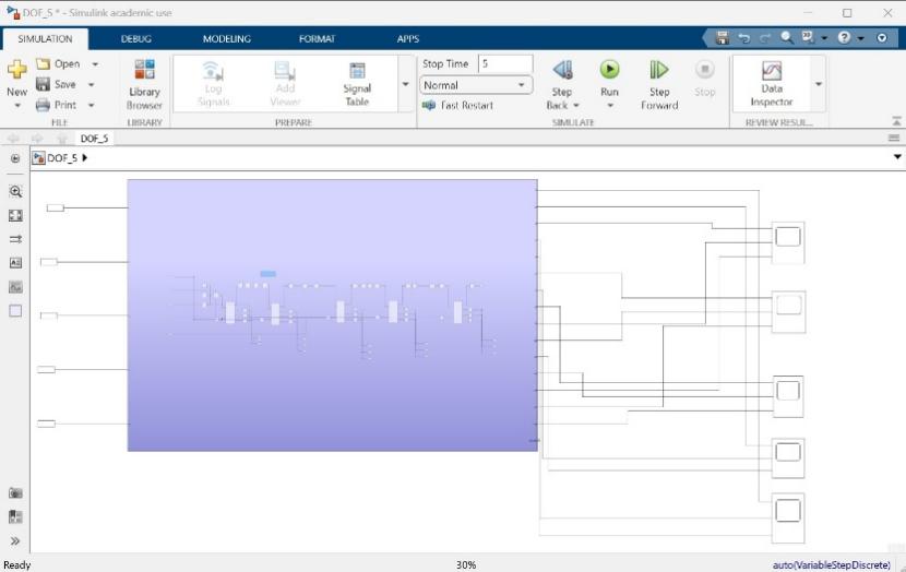
Figure 5. The 5-DOF robotic system in Simulink

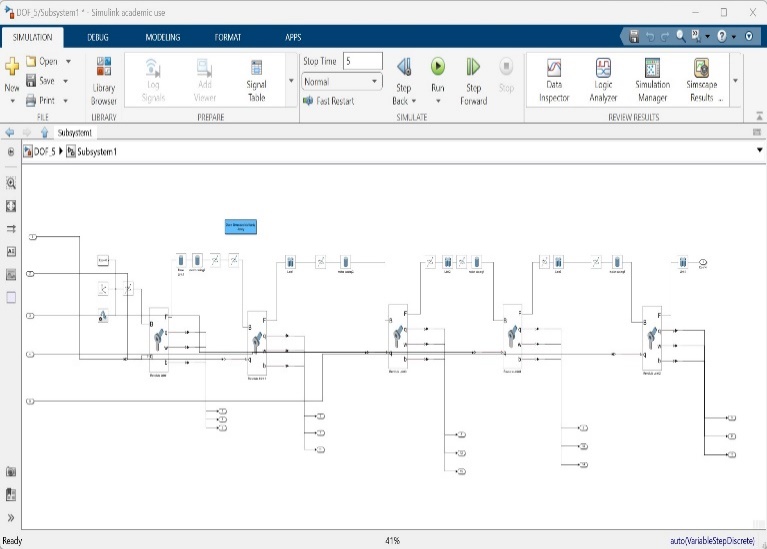
Figure 6. The 5-DOF robotic system in Simulink

The PID control loop in Simulink works by receiving continuous feedback on the end-effector’s orientation (the tilt and rotation angles) and comparing it to the desired reference (keeping the container's z-axis aligned with the global z-axis). The error between the current orientation and the target orientation generates control signals that adjust the end-effector's two joints (joints 4 and 5).

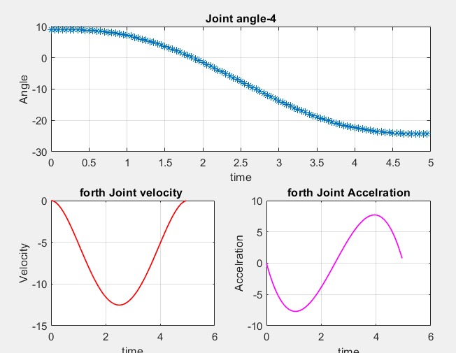
Figure 7. Joint angle 4 in Simulink

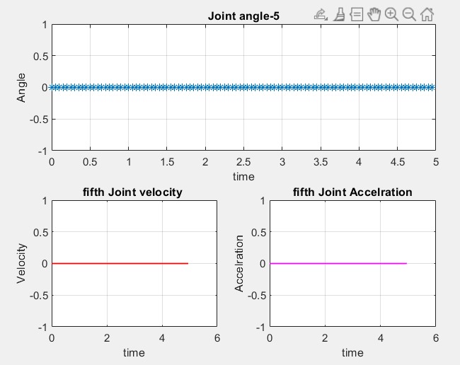
Figure 8. Joint angle 5 in Simulink

Proportional Control (P): Provides an immediate response to orientation errors. If the end-effector tilts, the proportional term applies a correction proportional to the magnitude of the error, keeping the response swift and direct.

Integral Control (I): Addresses accumulated errors over time to ensure that any minor deviations in the container’s orientation are corrected, ensuring long-term stability.

Derivative Control (D): Helps predict future errors based on the rate of change, adding damping to the system and ensuring smooth corrective movements without overshooting.

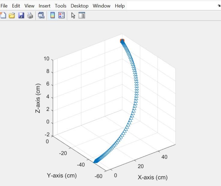
Figure 9. End effector trajectory

3.3. Simulink vs. Simscape: Control and Kinematics

In this project, the distinction between the roles of Simulink and Simscape is clear. Simscape focuses purely on the robot's kinematics, providing accurate modeling of the robot’s physical structure, joint movements, and the trajectory-following behavior of the 3-DOF arm and the 2-DOF end-effector. Simscape models how the robot should move but does not implement any dynamic control for keeping the container upright.

The dynamic control is handled in Simulink, where the PID controller adjusts the orientation of the end-effector. Simulink simulates the real-time feedback system required to correct the container's orientation and maintain balance. This integration allows for the simulation of the robot's full behavior, combining the physical accuracy of Simscape's kinematic model with Simulink’s control logic.”

4. Results and Discussion

The key challenge is maintaining the liquid's stability as the robot arm follows its trajectory. The 2-DOF end-effector provides the flexibility to adjust the container’s orientation, while the PID controller in Simulink ensures that these adjustments are made in real time to prevent spillage.

In the spherical pendulum model, the r parameter, defined as the ratio of ℓ, which represents the length of the rod connecting the end-effector, to h, which is the height of the container or end-effector, governs the system’s dynamic behavior. Using a similar PID controller in Simulink, different values of r result in varying responses in terms of stability and movement, directly impacting the trajectory and balancing of the liquid in the container. Nevertheless, the resulting angle and distance traveled for different values of r follow the same pattern, validating the pendulum model in achieving spill-free performance.

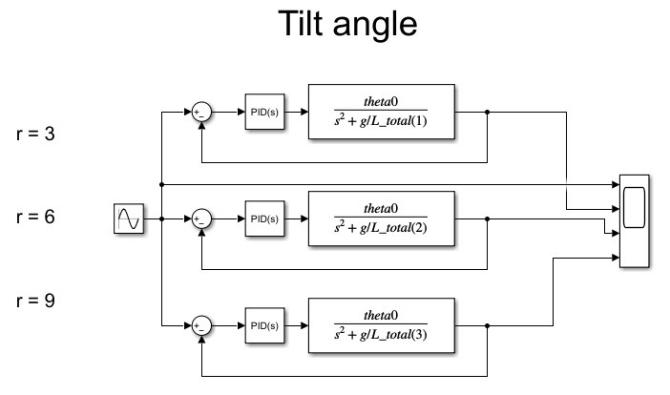
Figure 10. Simulation with PID for tilt angle with different values of r

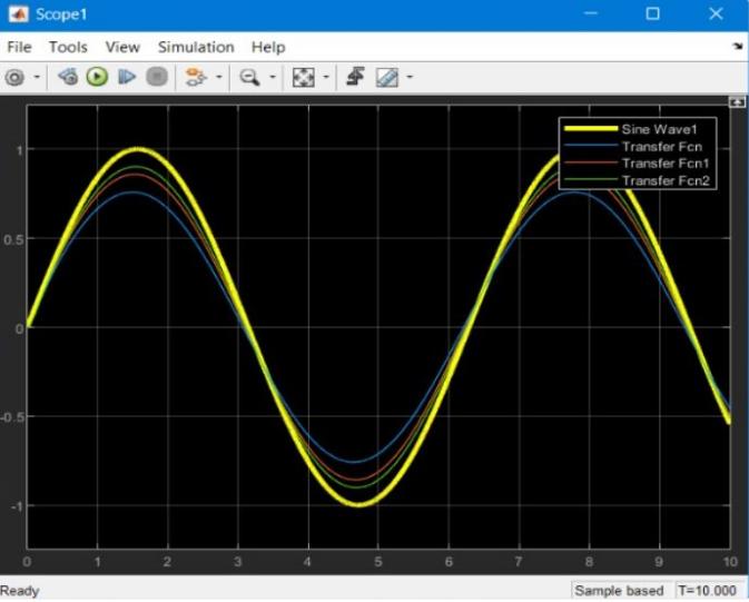
Figure 11. Tilt angle with different values of r

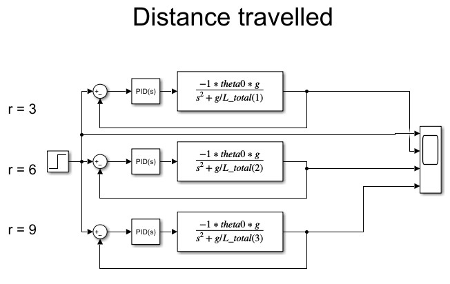
Figure 12. Simulation with PID for distance traveled with different values of r

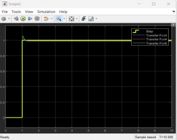
Figure 13. Spherical pendulum parameters

The simulation demonstrates that by using a well-tuned PID controller, the system can keep the container’s z-axis aligned with the global z-axis throughout the robot’s motion, even during sharp turns or rapid accelerations. This real-time balancing ensures that the liquid remains stable, effectively decoupling the robot’s position control (handled by Simscape) from the orientation control (handled by Simulink).

5. Limitations of the Work

The limitations of the work include:

Simplified Dynamic Model: The robot and liquid container system uses a simplified kinematic and dynamic model that does not account for all real-world factors, such as friction, vibration, and joint backlash, which could affect the accuracy of the end-effector's motion and liquid stability.

Assumption of Ideal PID Tuning: The PID controller assumes ideal tuning parameters. In practical scenarios, tuning might be more complex due to nonlinearities in the system, leading to potential instability or slower response times under different load conditions or trajectories.

Neglecting Fluid Dynamics: The model assumes that the liquid remains stable based solely on the container's orientation. However, real fluid dynamics, such as sloshing or surface tension effects, are not considered, which could impact the system's behavior during rapid movements or sharp turns.

Hardware Implementation Constraints: The simulation in Simulink and Simscape provides an idealized environment. When translating the design to a physical robot, limitations in hardware, such as actuator precision, sensor accuracy, and real-time processing delays, might affect performance and balancing capabilities.

Scalability and Flexibility: The model focuses on a specific 5-DOF robotic configuration and design. Adapting the system to different configurations with varying degrees of freedom or end-effector tools may require modifications to both the kinematic and control models.

6. Summary

In summary, this project leverages both Simscape and Simulink to design and control a 5-DOF robot capable of transporting a liquid-filled container without spillage. The kinematics of the robot are modeled in Simscape, providing an accurate simulation of the arm and end-effector’s physical movements. Meanwhile, the PID controller in Simulink manages the orientation of the end-effector, ensuring that the container stays upright throughout the robot's motion. This integration of kinematic modeling and dynamic control highlights the power of using both Simscape and Simulink to simulate and control complex robotic systems.

Acknowledgment

The completion of this research paper would not have been possible without the guidance of Professor Quan Nguyen at the University of Southern California and Zella Weizhe Ni at Columbia University.

References

[1]. Christian, Huygens, “Horologium Oscillatorium,” 17th CenturyMaths, March 2009.
[2]. Rafael I, Cabral Muchacho, Riddhiman Laha, Luis F.C. Figueredo, and Sami Haddadin, “A Solution to Slosh-free Robot Trajectory Optimization. Munich Institute of Robotics & Machine Intelligence.”
[3]. L. Moriello, L. Biagiotti, C. Melchiorri, and A. Paoli, “Manipulating liquids with robotics: A sloshing-free solution.” Control Engineering Practice, vol. 78, 2018, pp. 129-141.
[4]. Mihai Crenganis, Alexandru Barsan, Melania Tera, and Anca Chicea, “Dynamic analysis of a five degree of freedom robotic arm using MATLAB-Simulink Simscape,” MATEC Web of Conferences, 2021, pp 343.
[5]. Darina Hroncova, Lubica Mikova, Ivan Virgala, Erik Prada, “Kinematics of two link manipulator in Matlab/Simulink and MSC Adams / View Software,” MM Science Journal, October 2021, pp 4749.
[6]. Robert Barsanti, “Teaching PID Controller Design Using Matlab,” ASEE Southeast Section Conference, 2022.
Cite this article
Wang,J.;Ren,Y.;Zhao,J.;Lian,J. (2025). Spill-free Robotic Arm Based on Pendulum Model. Applied and Computational Engineering,131,202-211.
Data availability
The datasets used and/or analyzed during the current study will be available from the authors upon reasonable request.
Disclaimer/Publisher's Note
The statements, opinions and data contained in all publications are solely those of the individual author(s) and contributor(s) and not of EWA Publishing and/or the editor(s). EWA Publishing and/or the editor(s) disclaim responsibility for any injury to people or property resulting from any ideas, methods, instructions or products referred to in the content.
About volume
Volume title: Proceedings of the 2nd International Conference on Machine Learning and Automation
© 2024 by the author(s). Licensee EWA Publishing, Oxford, UK. This article is an open access article distributed under the terms and
conditions of the Creative Commons Attribution (CC BY) license. Authors who
publish this series agree to the following terms:
1. Authors retain copyright and grant the series right of first publication with the work simultaneously licensed under a Creative Commons
Attribution License that allows others to share the work with an acknowledgment of the work's authorship and initial publication in this
series.
2. Authors are able to enter into separate, additional contractual arrangements for the non-exclusive distribution of the series's published
version of the work (e.g., post it to an institutional repository or publish it in a book), with an acknowledgment of its initial
publication in this series.
3. Authors are permitted and encouraged to post their work online (e.g., in institutional repositories or on their website) prior to and
during the submission process, as it can lead to productive exchanges, as well as earlier and greater citation of published work (See
Open access policy for details).