1. Introduction

In recent years, with the rapid development of the national economy, the scale of the city continues to expand, more and more high-rise buildings and urban subway construction, deep foundation pit engineering has become an indispensable part. In particular, the city is rich in groundwater resources, which must be affected by groundwater during the excavation of foundation pits. Groundwater is buried deep underground, and there are many influencing factors, which causes great trouble to the study of groundwater dynamics [1].

At present, the prediction of groundwater level mainly includes traditional theoretical methods [2,3], numerical simulation methods [4,5] and artificial intelligence methods [6,7]. The better prediction effect is to use historical water level to establish a combined prediction model through statistics and neural network [8]. Neural network algorithms, such as ANN [9], ANFIS [10], GP [11], LSTM [12] and STGCN [13], do not require various physical parameters. These algorithm models are widely used in groundwater prediction research.

There are a large number of on-site monitoring data for us to excavate in the foundation pit project. The feedback of monitoring data is conducive to grasping the dynamic changes of water level in the foundation pit area in real time, adjusting the deployment of dewatering projects, and ensuring the safety of foundation pit excavation. In this paper, based on the field monitoring data of a subway dewatering project in Shenyang, the time domain prediction of foundation pit dewatering water level based on STGCN network, the spatial prediction of foundation pit dewatering water level based on Kriging interpolation optimized by Dupuit dewatering formula, and the spatio-temporal prediction of foundation pit dewatering water level based on STGCN and improved Kriging are modeled and analyzed.

2. Data preprocessing and distribution characteristics

2.1. The temporal distribution characteristics of groundwater depth in the study area

The water level change curve of 182 periods in 6 monitoring wells around the foundation pit is shown in Fig.1. The results of each monitoring sequence show that the water level change in the study area as a whole shows a trend from sharp to slow, and then with the increase of precipitation wells, the water level drops faster, the water level changes intensified, and finally the groundwater recharge and discharge reached a relative balance, and the water level gradually stabilized.

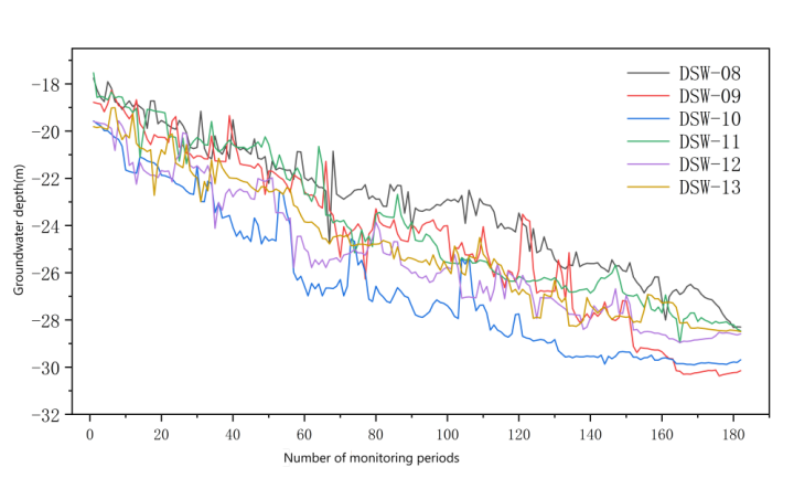
Figure 1: Water level change of monitoring Wells in stage 182

2.2. Spatial distribution characteristics of groundwater depth in the study area

Similar to the time distribution characteristics, under the action of group wells, the water level distribution in the surrounding area of the foundation pit also has certain spatial characteristics. Here, the foundation pit is divided into the following 8 areas, as shown in Figure 2.The box line statistics of 48 wells in the study area for 50 periods of data at the same time period are shown in Figure 3.It can be seen from the figure that the spatial distribution of groundwater level depth fluctuates around the edge of the foundation pit

.

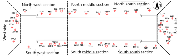
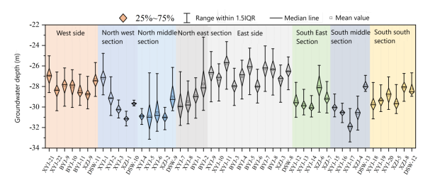
Figure 2: Schematic diagram of foundation Figure 3: Monitoring data box diagram of 48

pit area division Wells

2.3. Error evaluation index

Because the water level prediction problem is a typical nonlinear regression problem, the evaluation indexes of mean absolute error ( MAE ), root mean square error ( RMSE ) and mean absolute percentage error ( MAPE ) are selected to evaluate the regression effect.

3. Research methods

3.1. Time-domain prediction of foundation pit dewatering water level based on STGCN network

(1)Spatio-temporal convolution block captures the spatio-temporal characteristics of sequence.

The spatiotemporal convolution block captures the temporal characteristics of water level depth through the gated convolution layer, and captures the spatial characteristics of water level depth through the spatial map convolution layer. The spatio-temporal convolution block ( ST-Conv block ) is shown in Figure 4.

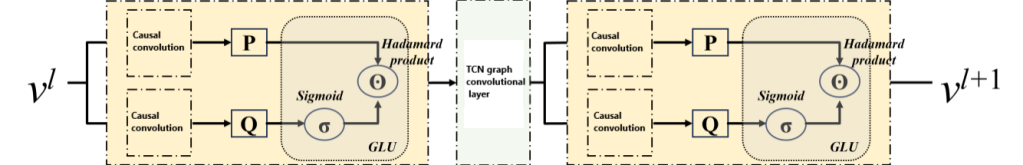
Figure 4: Schematic diagram of spatiotemporal convolution block

(2) The overall framework of STGCN model

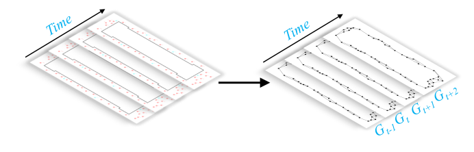
By constructing the spatio-temporal sequence data of each logging into a sequence diagram structure data with spatio-temporal attributes, the monitoring information is arranged according to the time series, so that the monitoring information becomes a dynamic time series signal, as shown in Fig.5.The STGCN water level prediction model can simultaneously predict the water level changes of all measuring points in the group well dewatering system, which greatly improves the practicability of the actual water level prediction task. The STGCN network structure is shown in Figure 6.

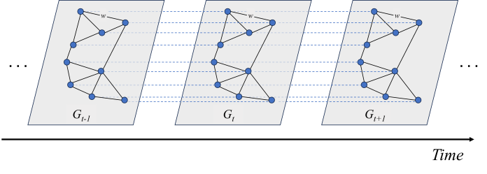
(a) Network structure of some wells on the east side of the foundation pit (b) Study the network structure of all wells in the research area

Figure 5: Network structure of sequential group Wells

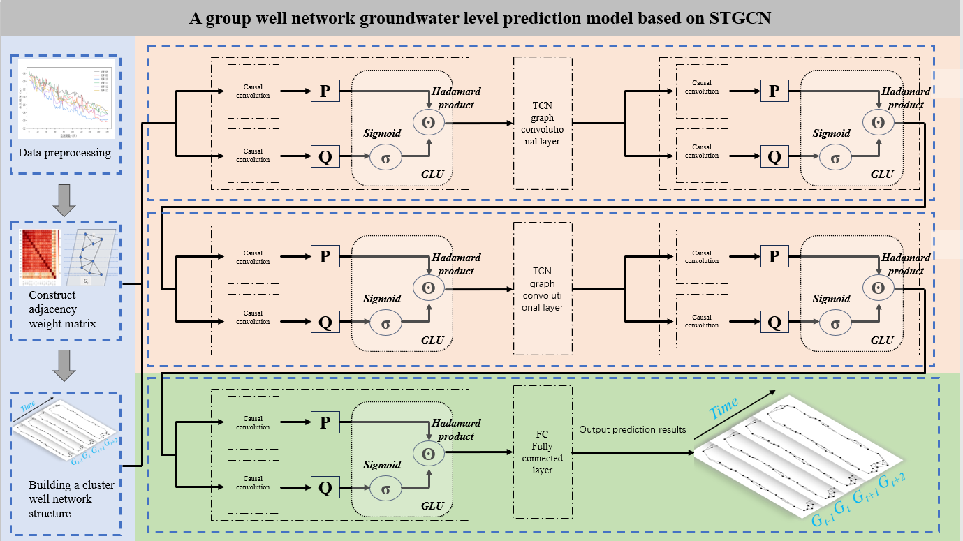
Figure 6: Flowchart of STGCN network structure

3.2. Analysis of dewatering mechanism of foundation pit group wells

(1) Dupuit stable well flow model

The Dupuit stable well flow model makes the following assumptions on the soil layer information in the group well precipitation area :

①The thickness of each aquifer in the precipitation area is consistent, isotropic and homogeneous, and the floor of the aquiclude is horizontal and has no lateral deformation in the horizontal direction.

②Compared with the influence range of precipitation, the influence of the radius of precipitation well is negligible.

③There is no vertical seepage supply and evaporation discharge ;

④The groundwater seepage conforms to Darcy 's law.

(2) Well group superposition theory

When multiple dewatering wells in the same aquifer are dewatering at the same time, the water level change of any well in the well group is usually composed of two parts : one is the water level change caused by the pumping of the well itself ; the other part is the water level change caused by the working of other wells in the well group system at the location of the well. This effect is called the interference well group effec.

3.3. Spatial prediction of foundation pit dewatering water level based on Kriging interpolation

(1) The basic principle of Kriging interpolation

Kriging interpolation needs to meet the two constraints of linear unbiased estimation and minimum variance expectation.

①Linear unbiased estimation refers to the mathematical expectation of the difference between the true value \( Z({x_{0}}) \) and the estimated value \( {Z^{*}}({x_{0}}) \) of any point \( {x_{0}} \) to be interpolated is 0, that is, the following equation :

\( E[{Z^{*}}({x_{0}})-Z({x_{0}})]=0\ \ \ (1) \)

②The minimum estimated variance means that the variance of the true value \( Z({x_{0}}) \) and the estimated value \( {Z^{*}}({x_{0}}) \) of all the interpolation points \( {x_{0}} \) is the smallest, that is, satisfies the formula 16.

\( J=min(Var[{Z^{*}}({x_{0}})-Z({x_{0}})])\ \ \ (2) \)

(2) Dupuit optimization Kriging interpolation semi-variance function

According to the basic principle of Kriging interpolation, the core equation of Kriging interpolation method is:

\( {Z^{*}}({x_{0}})=\sum _{i=1}^{n} {λ_{i}} Z({x_{i}})\ \ \ (3) \)

From the solution matrix of the weight coefficient \( {λ_{i}} \) in Equation 17, it can be seen that the \( {λ_{i}} \) value is related to the semi-variance function \( {y_{ij}} \) and the equivalent form of the semi-variance function is :

\( {r_{ij}}=E[{({z_{i}}-{z_{j}})^{2}}]/2\ \ \ （4） \)

It is more scientific to use the Dupuit precipitation formula that considers more influencing factors to fit a semi variance function \( γ=γ(d,{H_{0}},Q,k,R) \) instead of a semi variance fitting function \( y=y(d) \) that only considers distance effects.

4. Results analysis

The STGCN network simultaneously predicts all measuring points. Figure 7 below shows the comparison between the predicted results of 42 precipitation wells and 6 monitoring wells in the study area predicted by the STGCN model and the actual monitoring results. The average error of the prediction results of the STGCN model at the monitoring well is 0.34 m, and the average error percentage is 1.17 %. The average error of the prediction results at the precipitation well is 0.30 m, and the average error percentage is 1.05.

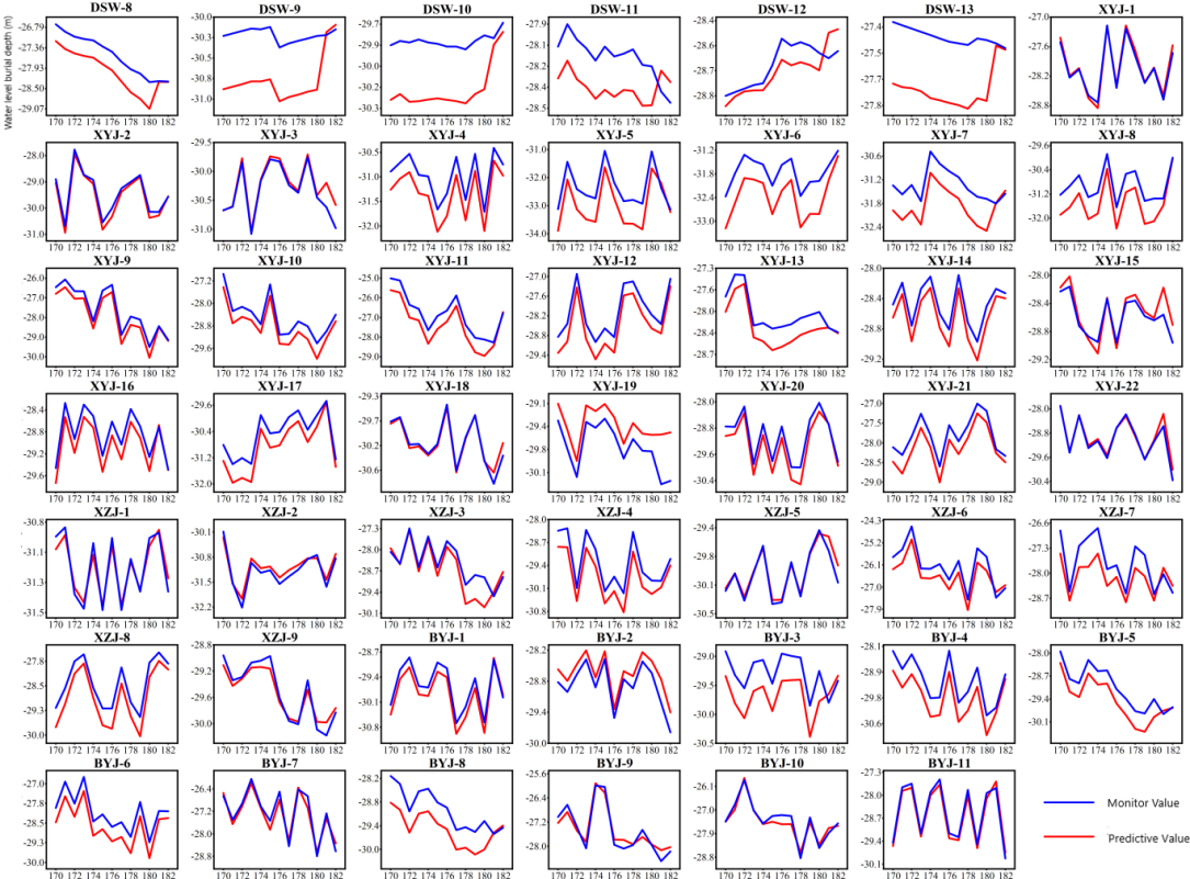
Figure 7: Comparison curves of all Wells predicted and measured

In the position of 6 monitoring wells, the average error of OK method is 1.06 m, and the error percentage is 3.79 %. The average error of IDW method is 1.15 m, and the error percentage is 3.64 %. The average error of the SP method is 1.29 m, and the error percentage is 4.64 %. In terms of interpolation prediction performance, the improved Kriging interpolation method proposed in this paper increases by 33.02 %, 38.26 % and 44.96 % respectively. The above performance evaluation indicators are quantified as shown in Figure 8.

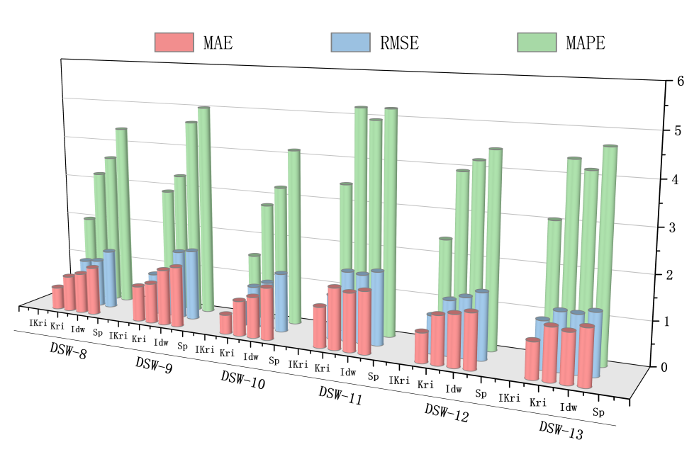
Figure 8: Comparison of accuracy evaluation indexes of four interpolation methods

According to the above research, the prediction results of the water level distribution in the study area based on the STGCN-Kriging interpolation prediction method are in good agreement with the actual distribution of the water level in reality. For example, see Figure 9 below.

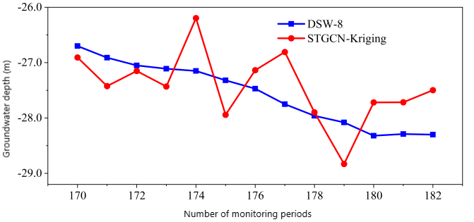
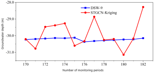
(a)Interpolation prediction results at DSW-8 logging site (b)Interpolation prediction results at DSW-9 logging site

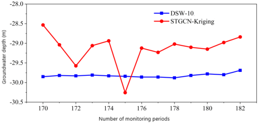
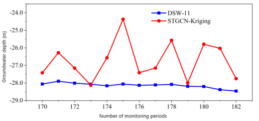
(c)Interpolation prediction results at DSW-10 logging site (d)Interpolation prediction results at DSW-11 logging site

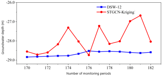
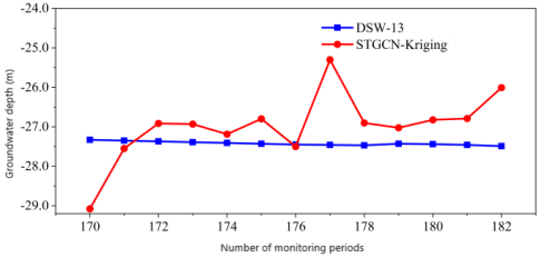
(e)Interpolation prediction results at DSW-12 logging site (f)Interpolation prediction results at DSW-13 logging site

Figure 9: Comparison between STGCN-kriging prediction interpolation and actual situation

It can be seen from the diagram that the STGCN-Kriging interpolation prediction curve always fluctuates around the monitoring curve. The average error of the interpolation prediction results is 0.79 m, and the relative error percentage is 2.79 %. The STGCN-Kriging spatio-temporal prediction is carried out for the whole region. On the whole, it provides valuable water level information for the area not covered by measuring points, and provides continuous water level distribution map in time and space for the whole observation area.

5. Conclusion

The deep learning method and Dupuit group well precipitation formula are introduced to optimize the neglect of spatial-temporal correlation in Kriging interpolation, and an improved Kriging interpolation method is proposed to predict the spatial domain of water level. Finally, the STGCN network is combined with the improved Kriging interpolation method to propose a prediction model that can predict the spatial and temporal distribution of water level in time-space domain. The main conclusions are as follows :

(1)The groundwater depth in the study area showed a trend of ' acute-slow-acute-slow-stable ' in the time distribution. In the spatial distribution, the water level on the north and south sides of the long side of the foundation pit decreases greatly, and the water level on the east and west sides of the short side decreases slightly.

(2)The STGCN network model is built, and the characteristics of the graph convolution network and the gated convolution network are used to predict all the measuring points at the same time. The prediction efficiency is better than the model that predicts each measuring point one by one.

(3)The semi-variance function in Kriging interpolation is optimized by combining deep learning algorithm and Dupuit precipitation formula, which is more in line with the actual change law of groundwater.

References

[1]. Chen Fei, Xu Xiangyu,Yang Yan, et al. Evolution trend and influencing factors of groundwater resources in China [J]. Advances in Water Science, 2020, 31 (06): 811-819.(in Chinese)
[2]. Neuman S P. Theoretical derivation of Darcy's law[J]. Acta mechanica, 1977, 25(3): 153-170.
[3]. Hantush M S. On the validity of the Dupuit‐Forchheimer well‐discharge formula[J]. Journal of Geophysical Research, 1962, 67(6): 2417-2420.
[4]. Mahmoudpour M, Khamehchiyan M, Nikudel M R, et al. Numerical simulation and prediction of regional land subsidence caused by groundwater exploitation in the southwest plain of Tehran, Iran[J]. Engineering Geology, 2016, 201: 6-28.
[5]. Min Liantai.Prediction of temperature distribution of groundwater by mathematical simulation-heat transfer of steady flow in confined aquifer [J]. Prospecting Technology, 1979, (06): 82 +76.(in Chinese)
[6]. Hussein E A, Thron C, Ghaziasgar M, et al. Groundwater prediction using machine-learning tools[J]. Algorithms, 2020, 13(11): 300.
[7]. Liu Di, Yu Zhongbo, Lu Haishen, et al. Prediction of groundwater level change based on SVM-EnKF bidirectional data assimilation [J]. Hydrology, 2023, 43 (06): 58-65.(in Chinese)
[8]. Nourani V, Ejlali R G, Alami M T. Spatiotemporal groundwater level forecasting in coastal aquifers by hybrid artificial neural network-geostatistics model: a case study[J]. Environmental Engineering Science, 2011, 28(3): 217-228.
[9]. Sahoo S, Jha M K. Groundwater-level prediction using multiple linear regression and artificial neural network techniques: a comparative assessment[J]. Hydrogeology Journal, 2013, 21(8): 1865.
[10]. Shirmohammadi B, Vafakhah M, Moosavi V, et al. Application of several data-driven techniques for predicting groundwater level[J]. Water Resources Management, 2013, 27: 419-432.
[11]. Fallah-Mehdipour E, Haddad O B, Mariño M A. Prediction and simulation of monthly groundwater levels by genetic programming[J]. Journal of Hydro-Environment Research, 2013, 7(4): 253-260.
[12]. Hou Jinxiao, Huang Linxian, Hu Xiaonong, et al.Forecasting application of karst groundwater level in Baotu Spring based on EMD-LSTM coupling model [J]. Journal of Water Resources and Water Engineering, 2023, 34 (04): 92-98.(in Chinese)
[13]. Yu Yufeng, Li Wei, Li Ke, et al. Real-time correction of flood forecasting error based on STGCN [J]. Hydrology, 2022, 42 (05): 35-40.(in Chinese)
Cite this article
Zhao,C.;Huang,Z. (2025). Prediction of Foundation Pit Dewatering Water Level Based on Neural Network and Improved Kriging Interpolation. Applied and Computational Engineering,116,174-180.
Data availability
The datasets used and/or analyzed during the current study will be available from the authors upon reasonable request.
Disclaimer/Publisher's Note
The statements, opinions and data contained in all publications are solely those of the individual author(s) and contributor(s) and not of EWA Publishing and/or the editor(s). EWA Publishing and/or the editor(s) disclaim responsibility for any injury to people or property resulting from any ideas, methods, instructions or products referred to in the content.
About volume
Volume title: Proceedings of the 5th International Conference on Signal Processing and Machine Learning
© 2024 by the author(s). Licensee EWA Publishing, Oxford, UK. This article is an open access article distributed under the terms and
conditions of the Creative Commons Attribution (CC BY) license. Authors who
publish this series agree to the following terms:
1. Authors retain copyright and grant the series right of first publication with the work simultaneously licensed under a Creative Commons
Attribution License that allows others to share the work with an acknowledgment of the work's authorship and initial publication in this
series.
2. Authors are able to enter into separate, additional contractual arrangements for the non-exclusive distribution of the series's published
version of the work (e.g., post it to an institutional repository or publish it in a book), with an acknowledgment of its initial
publication in this series.
3. Authors are permitted and encouraged to post their work online (e.g., in institutional repositories or on their website) prior to and
during the submission process, as it can lead to productive exchanges, as well as earlier and greater citation of published work (See
Open access policy for details).