1. Introduction

The Markov Chain Monte Carlo (MCMC) method named by American physicist Metropolis et al [1, 2] was developed and proposed during the “Manhattan Project” to create the atomic bomb. Canadian statistician Hastings [3] and his Ph.D. student Peskun [4] overcame the dimensional bottleneck problem encountered by conventional Monte Carlo methods. They generalized the Metropolis algorithm and extended it as a statistical simulation tool, forming the Metropolis-Hastings algorithm.

Compared with the Metropolis method, the Metropolis-Hastings algorithm s a statistical simulation tool looks more professional. What is important is that the symmetrical proposal distribution function in Metropolis-Hastings algorithm is not necessary, so it is more flexible and convenient to apply [5, 6, 7].

2. Ease

2.1. Metropolis-Hastings algorithm

The Metropolis-Hastings algorithm is one of the most popular MCMC methods and is utilized to simulate a sequence of random samples, a Markov chain converging to a stationary target distribution \( π(∙) \) , which is difficult to sample directly. Let \( q({x_{t+1}}|{x_{t}}) \) denote the proposal probability that moves from \( {x_{t}} \) at time t to \( {x_{t+1}} \) at time t+1. The proposed distribution can facilitate the simulation of a Markov chain corresponding to the target distribution. The algorithm is implemented in the following steps:

Step 1: Initialize the current state \( {x_{t}} \) ;

Step 2: Generate a candidate \( x_{t+1}^{*} \) value from the proposal distribution \( q(x_{t+1}^{*}|{x_{t}}) \) ;

Step 3: Calculate the acceptance probability \( {α_{t}}({x_{t}},x_{t+1}^{*}) \) :

\( {α_{t}}({x_{t}},x_{t+1}^{*})=min\lbrace \frac{π(x_{t+1}^{*})q({x_{t}}|x_{t+1}^{*})}{π({x_{t}})q(x_{t+1}^{*}|{x_{t}})},1\rbrace \) (1)

Step 4: Generate \( {u_{t}} \) from a uniform distribution on [0, 1];

Step 5: If \( {u_{t}}≤{a_{t}} \) , accept the candidate value \( x_{t+1}^{*} \) and set \( {x_{t+1}}=x_{t+1}^{*} \) ; otherwise, reject the candidate value \( x_{t+1}^{*} \) and set \( {x_{t+1}}={x_{t}} \) ;

Step 6: Repeat Step 2 to Step 5 until a sample of the desired size N is obtained.

Based on the choice of the proposal distribution, the Independent Metropolis algorithm and Random-walk Metropolis algorithm (RWM) are two typical Metropolis-Hastings algorithms [8].

2.1.1. Independent Metropolis algorithm

In this case, the candidate value \( x_{t+1}^{*} \) is independent of the current state \( {x_{t}} \) , which is formed as

\( q(x_{t+1}^{*}|{x_{t}})=q({x_{t}}) \) ,

The acceptance probability \( {α_{t}}({x_{t}},x_{t+1}^{*}) \) is then modified to

\( {α_{t}}({x_{t}},x_{t+1}^{*})=min\lbrace \frac{π(x_{t+1}^{*})q({x_{t}})}{π({x_{t}})q(x_{t+1}^{*})},1\rbrace \) (2)

2.1.2. Random-walk Metropolis algorithm

The critical feature of RWM is that the candidate value \( x_{t+1}^{*} \) is centered distributedly on the current state \( {x_{t}} \) , i.e.

\( x_{t+1}^{*}={x_{t}}+\grave{o} \) ,

where \( \grave{o} \) is distributed symmetrically with mean zero. For example, the proposal value \( x_{t+1}^{*} \) given \( {x_{t}} \) is simulated from a normal distribution \( x_{t+1}^{*}|{x_{t}}~N({x_{t}},{σ^{2}}) \) . Therefore, the acceptance probability \( {α_{t}}({x_{t}},x_{t+1}^{*}) \) is simplified to

\( {α_{t}}({x_{t}},x_{t+1}^{*})=min\lbrace \frac{π(x_{t+1}^{*})}{π({x_{t}})},1\rbrace \) (3)

2.2. Application

2.2.1. Data and Model

In this paper, we study the number of widowed women with different number of children in Manchester, 2021, the data of which is shown in Table 1 and Figure 1.

Table 1: The numbers of widows with different number of children

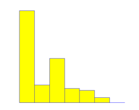
Figure 1: Histogram for the numbers of widows

We use a zero-inflated Poisson model based on the distribution in Figure 1. Let Y be the number of children per widowed woman. The data \( {y_{1}},{y_{2}},…,{y_{n}} \) are the observations corresponding to Table 1 [9], where n is the total number of widows and assumed independent and identically distributed from the following probability mass function:

\( f(y|λ,ε)=\begin{cases} \begin{array}{c} ε+(1-ε){e^{-λ}} y=0 \\ (1-ε)\frac{{λ^{y}}{e^{-λ}}}{y!} y=1,2,…,n \end{array} \end{cases} \) (4)

To predict the number of widows with different numbers of children using the zero-inflated Poisson distribution, we first estimate the values of \( λ \) and \( ε \) through the Metropolis-Hastings algorithms.

For simplicity, assume that both \( λ \) and \( ε \) have uniform priors. Thus, the posterior distribution for \( (λ,ε) \) is proportional to the following form:

\( f(λ,ε|y)∝\prod _{i=1}^{n} f({y_{i}}|λ,ε) \) (5)

Therefore, we obtain the target distribution of \( (λ,ε) \) :

\( π(λ,ε)=\prod _{i=1}^{n} f({y_{i}}|λ,ε) \) (6)

Based on the properties of zero-inflated Poisson distribution and the observed data, we initialize the value of \( λ \) and \( ε \) as follows:

\( \hat{ε}=f(0)=\frac{52}{n}=0.4952; \)

\( \hat{λ}=y/(1-ε ̂ )=2.3962,as EY=λ(1-ε) \) (7)

Subsequently, we shall produce sequences of \( λ \) and \( ε \) simulation with a sample size N=10000 by two different algorithms.

2.2.2. Independent Metropolis

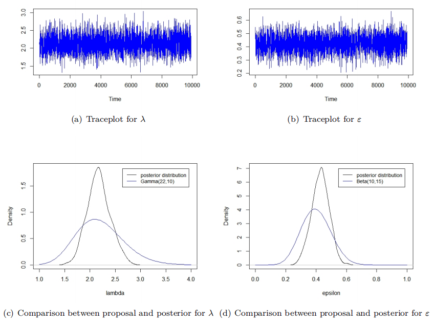
Figure 2: Independent Metropolis

According to the posterior distribution, we assume \( λ~Gamma({α_{1}},{β_{1}}) \) and \( ε~Beta({α_{2}},{β_{2}}) \) to be proposal distributions for \( λ \) and \( ε \) , respectively. Thus, we have proposal probability \( {q_{1}}(λ) \) and \( {q_{2}}(ε) \) :

\( {q_{1}}(λ)=\frac{β_{1}^{{α_{1}}}}{Γ({α_{1}})}{λ^{{α_{1}}-1}}{e^{-{β_{1}}λ}} \) (8)

\( {q_{2}}(ε)=\frac{1}{B}{ε^{{α_{2}}-1}}(1-ε{)^{{β_{2}}-1}} \) (9)

In this case, the acceptance probability \( {α_{t}}\lbrace ({λ_{t}},{ε_{t}}),(λ_{t+1}^{*},ε_{t+1}^{*})\rbrace \) is

\( {α_{t}}=min\lbrace \frac{π(λ_{t+1}^{*},ε_{t+1}^{*})}{π({λ_{t}},{ε_{t}})}\cdot \frac{{q_{1}}({λ_{t}})}{{q_{1}}(λ_{t+1}^{*})}\cdot \frac{{q_{2}}({ε_{t}})}{{q_{2}}(ε_{t+1}^{*})},1\rbrace \) (10)

To confirm a specific distribution, we need to choose reasonable parameters \( {α_{1}},{β_{1}},{α_{2}},{β_{2}} \) in the proposal probabilities \( {q_{1}}(λ) \) and \( {q_{2}}(ϵ). \) The key point in this selection is to ensure that the proposal distributions for \( λ \) and \( ϵ \) are both close to the posterior distribution and exhibit greater dispersion than the posterior distribution [10].

For example, \( {q_{1}}(λ)∼N({α_{1}},β_{1}^{2}) \) and \( {q_{2}}(ϵ)∼N({α_{2}},β_{2}^{2}) \) are possible choices. Figure 2(a) and Figure 2(b) show the trace plots for the simulations of \( λ \) and \( ϵ \) , respectively. Both trace plots in Figure 2 illustrate stationary Markov chains that move quickly, indicating that the algorithm performs effectively. Additionally, the comparison between the proposal and posterior distributions for \( λ \) and \( ϵ \) in Figures 2(c) and 2(d) demonstrates that the proposals not only have means similar to the posteriors but also exhibit greater dispersion than the posterior distributions. These characteristics confirm that the chosen parameters for the proposal distributions are appropriate and contribute to the effectiveness of the algorithm.

2.2.3. Random-walk Metropolis

Based on the RWM algorithm, Normal proposal distribution is assumed for both \( λ \) and \( ε \) . Therefore, we propose to sample \( {ε^{*}}~N(ε,σ_{ε}^{2}) \) and \( {λ^{*}}~N(λ,σ_{λ}^{2}) \) , where \( σ_{ε}^{2} \) and \( σ_{λ}^{2} \) represent the proposed variances for \( λ \) and \( ε \) , respectively. In this case, the acceptance probability is

\( {α_{t}}=min\lbrace \frac{π(λ_{t+1}^{*},ε_{t+1}^{*})}{π({λ_{t}},{ε_{t}})},1\rbrace \) (11)

Then tuning \( σ_{ε}^{2} \) and \( σ_{λ}^{2} \) is able to optimize the performance of the algorithm. We choose \( (σ_{λ}^{2},σ_{ε}^{2}) \) in different values (0.001, 0.0001), (0.2, 0.02), (2, 0.2), and all the implements of the first 1000 samples are shown in the Figure 3.

For the case \( (σ_{λ}^{2},σ_{ε}^{2})=(0.001, 0.0001) \) , most candidate values of \( λ \) and \( ε \) are accepted. However, the move in each step is very small. Thus it takes a long time for the Markov chains of \( λ \) and \( ε \) to explore and they do not converge to posterior distributions. \( (σ_{λ}^{2},σ_{ε}^{2})=(0.2, 0.02) \) is the other extreme case, where few candidate values of \( λ \) and \( ε \) in the moving are accepted. For the case \( (σ_{λ}^{2},σ_{ε}^{2})=(0.2, 0.02) \) , the traceplots show that both Markov chains move fast and appear to be converged and therefore, it is the optimal choice for the RWM algorithm.

2.2.4. Result and Analysis

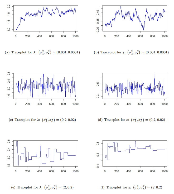
Figure 3: Random-walk Metropolis

Based on the samples of size N=10000 for \( λ \) and \( ε \) from two algorithms, we estimate the numbers of widows with different children in Manchester from the zero-inflated Poisson model using Monte-Carlo method. The results are summarized in Table 2 and shown in Figure 3 and Figure 4.

Table 2: Result

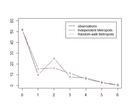
Figure 4: Comparison of result

We observe that both Independent Metropolis and RWM have good agreement on the numbers of widowed women with different numbers of children. Comparing with the observations, both algorithms provide accurate estimations for the number of widows with 0, 4, 5, and 6 children. However, there are large differences between the expected numbers and observations for cases that widowed women have 1, 2, 3 children.

3. Conclusion

In this paper, two variations of the Metropolis-Hastings algorithm—the Independent Metropolis and the Random-Walk Metropolis (RWM)—were applied to a zero-inflated Poisson model to estimate the distribution of widows with different numbers of children in Manchester. By adjusting the parameters within the algorithms, reasonable samples of the zero-inflated Poisson model parameters π and λ were obtained.

When comparing the predicted values (obtained from the model using the estimated parameters) with the observed values (actual data from Manchester), the model demonstrates a generally good fit. However, there is a noticeable gap between the predicted values and the observed values in specific cases, particularly for widows with 1, 2, or 3 children. This suggests that while the model performs adequately overall, the true distribution of the data may not be fully captured by the zero-inflated Poisson model.

To address these discrepancies, future studies could consider exploring alternative models, such as the Negative Binomial Zero-Inflated model, which may better account for overdispersion in the data and provide an improved fit to the observed values.

References

[1]. N. Metropolis and S. Ulam, “The monte carlo method,” Journal of the American statistical association, vol. 44, no. 247, pp. 335–341, 1949.
[2]. N. Metropolis, A. W. Rosenbluth, M. N. Rosenbluth, A. H. Teller, and E. Teller, “Equation of state calculations by fast computing machines,” The journal of chemical physics, vol. 21, no. 6, pp. 1087–1092, 1953.
[3]. W. K. Hastings, “Monte Carlo sampling methods using Markov chains and their applications,” Biometrika, vol. 57, no. 1, pp. 97–109, 1970.
[4]. P. H. Peskun, “Optimum monte-carlo sampling using markov chains,” Biometrika, vol. 60, no. 3, pp. 607–612, 1973.
[5]. A. Gelman, W. R. Gilks, and G. O. Roberts, “Weak convergence and optimal scaling of random walk metropolis algorithms,” The annals of applied probability, vol. 7, no. 1, pp. 110–120, 1997.
[6]. C. Andrieu, N. De Freitas, A. Doucet, and M. I. Jordan, “An introduction to mcmc for machine learning,”Machine learning, vol. 50, no. 1, pp. 5–43, 2003.
[7]. C. Robert and G. Casella, “A short history of markov chain monte carlo: Subjective recollections from incomplete data,” Statistical Science, vol. 26, no. 1, pp. 102–115, 2011.
[8]. Madrigal-Cianci, Juan P., Fabio Nobile, and Raul Tempone. "Analysis of a class of multilevel Markov chain Monte Carlo algorithms based on independent Metropolis–Hastings." SIAM/ASA Journal on Uncertainty Quantification 11.1 (2023): 91-138.
[9]. Teixeira, J. S., et al. "A new adaptive approach of the Metropolis-Hastings algorithm applied to structural damage identification using time domain data." Applied Mathematical Modelling 82 (2020): 587-606.
[10]. Choi, Michael CH, and Lu-Jing Huang. "On hitting time, mixing time and geometric interpretations of metropolis–hastings reversiblizations." Journal of Theoretical Probability 33.2 (2020): 1144-1163.
Cite this article
Chen,Y. (2025). Metropolis-Hastings Algorithms based on a Zero-inflated Poisson Model. Applied and Computational Engineering,116,187-193.
Data availability
The datasets used and/or analyzed during the current study will be available from the authors upon reasonable request.
Disclaimer/Publisher's Note
The statements, opinions and data contained in all publications are solely those of the individual author(s) and contributor(s) and not of EWA Publishing and/or the editor(s). EWA Publishing and/or the editor(s) disclaim responsibility for any injury to people or property resulting from any ideas, methods, instructions or products referred to in the content.
About volume
Volume title: Proceedings of the 5th International Conference on Signal Processing and Machine Learning
© 2024 by the author(s). Licensee EWA Publishing, Oxford, UK. This article is an open access article distributed under the terms and
conditions of the Creative Commons Attribution (CC BY) license. Authors who
publish this series agree to the following terms:
1. Authors retain copyright and grant the series right of first publication with the work simultaneously licensed under a Creative Commons
Attribution License that allows others to share the work with an acknowledgment of the work's authorship and initial publication in this
series.
2. Authors are able to enter into separate, additional contractual arrangements for the non-exclusive distribution of the series's published
version of the work (e.g., post it to an institutional repository or publish it in a book), with an acknowledgment of its initial
publication in this series.
3. Authors are permitted and encouraged to post their work online (e.g., in institutional repositories or on their website) prior to and
during the submission process, as it can lead to productive exchanges, as well as earlier and greater citation of published work (See
Open access policy for details).