1. Introduction

In modern society, artificial intelligence (AI) is increasingly integrated into daily applications, especially in technology, with innovations like Chat-GPT and bio-inspired robotics. These tools enable efficient data transmission to AI for analysis and model creation. Machine learning has advanced fields such as medicine, transportation, and education. However, as these industries evolve, the demand for accurate and efficient machine-learning models grows. This manuscript examines key supervised learning algorithms, including linear regression, decision trees, and neural networks, assessing their performance across various data types and applications. Results show that algorithm suitability varies by task, and model prediction accuracy is influenced by data quality, selection, algorithm choice, loss function, and internal structure. This work aims to clarify the architecture of supervised machine learning and its theoretical underpinnings, promoting broader practical applications. Supervised learning is poised to tackle more complex challenges in the future.

2. Overview of Supervised Learning Algorithms

2.1. Classification of Common Supervised Learning Algorithms

Supervised learning is a fundamental algorithm in machine learning, crucial for technological advancement. It entails training models on historical data to forecast future outcomes, partitioning data into training and test sets. The model learns from the training set, adjusting parameters based on input and output variables, while the test set assesses prediction accuracy. Techniques such as linear regression, decision trees, and neural networks are esteemed and widely utilized in finance, medical imaging, and image classification. This paper evaluates the performance of these algorithms across diverse data characteristics and scales, utilizing mathematical models to clarify their principles. Subsequently, it analyzes loss functions and optimization algorithms, exploring the characteristics and contexts of various loss functions.[1] Finally, evaluating the prediction accuracy and stability of various algorithms in different data characteristics. Through the application of supervised learning in practical scenarios, it can be utilized to forecast material properties and enhance these properties to reduce production costs.[2] Also, it can apply to the prediction of postpartum depression after the women give birth so that they can get treatment.

2.2. Working Principle and Basic Process of Supervised Learning Algorithm:

The three primary categories of supervised learning are linear regression, decision trees, and neural networks. Linear regression, a fundamental statistical model, is widely applied in numerous real-world contexts. The linear function, depicting the direct relationship between dependent and independent variables, is familiar to many.[3]For linear regression, the \( γ \) variable is the \( γ \) dependent variable(label or target in machine learning). The \( χ \) variable is the independent variable(feature or input variable). Noted, only one \( γ \) variable but the models can have more than one \( χ \) variable which is constructed to multiple linear regression. In linear regression, employing a linear function to fit a model to the dataset comprising the independent variable ( \( χ \) ) and the dependent variable ( \( γ \) ). Subsequently, utilizing this model to forecast the \( γ \) value based on a new \( χ \) variable.[3] A decision tree classifies data through conditions, utilizing nodes as features, branches as outcomes, and leaves as results. It differentiates nodes based on data attributes, leading to distinct terminal outcomes. Once all data points are categorized, unnecessary nodes are pruned to enhance purity. New data traverses from nodes to leaves to generate predictions. The decision tree yields both categorical and numerical results: Classification Prediction determines data categories, such as classifying an email as spam or legitimate, while Regression Prediction offers quantitative forecasts. [4] Estimate property value by room count using a neural network, akin to a brain's structure. The common single-layer network includes an input layer ( \( χ \) variable), weights, and an output layer ( \( γ \) variable). It functions linearly with linearly separable data. Alternatively, it must employ activation functions like sigmoid, ReLU, and Leaky ReLU.[3]

3. Theoretical Basis of Supervised Learning Algorithms

3.1. Mathematical Model and Theoretical Framework: Using Mathematical Formulas to Explain the Core Principles of the Algorithm:

For the next session, This article will explain the core principle of the three algorithms with mathematical formulas. Linear regression is one of the most common and widely used algorithms. The formula is similar to a linear function. The function is

\( {γ_{}}≈{β_{0}}+{β_{1}}{χ_{}} \) (1)

This \( ≈ \) can be seen as an approximate model. The Y is the \( γ \) variable which is the label of the data. The \( {χ_{}} \) is the \( {χ_{}} \) variable which is the feature or the independent variable of the data. \( {β_{0}} \) and \( {β_{1}} \) are parameters or coefficients of this function and they are unknown. The \( {β_{0}} \) is the intercept of this function. When \( χ \) is equal to zero, the function hits the \( γ \) -axis. The \( {β_{1}} \) is the slope of this function. After using our training data to get estimates \( \hat{{β_{0}}} \) and \( \hat{{β_{1}}} \) . The function of the prediction will be

\( \hat{γ}≈\hat{{β_{0}}}{+ \hat{{β_{1}}}χ_{}} \) (2)

The little hat means predicted. The solution to finding out two parameters is using the function of both the \( γ \) hat and the normal \( γ \) . For the ith value of \( χ \) , the normal \( γ \) function can be written as

\( {γ_{i}}≈{β_{0}}+{β_{1}}{χ_{i}} \) (3)

and the predicted function can be written as

\( \hat{{γ_{i}}}≈\hat{{β_{0}}}{+ \hat{{β_{1}}}{χ_{i}}_{}} \) (4)

Then, \( ϵi \) represents the difference of \( {γ_{i}} \) and \( \hat{{γ_{i}}} \) . The square of the difference is the residual sum of the square. So the residual sum of the square(RSS) is

RSS = \( ϵi \) + \( ϵ_{2}^{2} \) + …+ \( ϵ_{i}^{2} \) (5)

Each one can be written as [3]:

RSS = \( \sum _{i=1}^{n}({γ_{1}}-\hat{{β_{0}}}- \hat{{β_{1}}}{χ_{i}}) \) (6)

After using calculus and math calculation, the values are:

\( {β_{1}} \) = \( (\sum _{i=1}^{n}({χ_{1}}-\overline{χ})({γ_{i}}-\overline{γ}))÷(\sum _{i=1}^{n}{({χ_{1}}-\overline{χ})^{2}}) \) (7)

\( {β_{0}} \) = \( (\overline{γ}-{β_{1}}\overline{χ}) \) (8)

\( \overline{χ} \) and \( \overline{γ} \) are the sample mean of the given data. It can solve the parameters based on the equation. The math equation for the decision tree is easy to understand. Let’s say there is a data set called D. In the previous section, The article talked about splitting each node based on selecting a feature and finding a threshold for that feature if it has a feature called \( χ \) and a threshold called t. After a time split. The new data set for the left and right sides are:

\( {D_{left}} \) = \( \lbrace ({χ_{i}},{γ_{1}})∈D|{χ_{i}}≤t\rbrace \) ;(9)

\( {D_{right}} \) = \( \lbrace ({χ_{i}},{γ_{1}})∈D|{χ_{i}} \gt t\rbrace \) ;(10)

For the first equation as an example. The “ \( ({χ_{i}},{γ_{1}})∈D \) ” represents the number of \( χ \) and \( γ \) are the elements of data set D. “ \( {χ_{i}}≤t \) ” represents the ith data point of \( χ \) is less or equal than the threshold t. For the neural network. Each neural network has three layers: the input layer, the hidden layer, and the output layer. Each layer connects to the next layer with a weight. For the ith item of \( χ \) (input layer). The equation is

\( γ \) = \( {ω_{i}}{χ_{i}} \) (11)

If the neural network is non-linear, the activation function will added to the equation such as sigmoid, ReLu, and Leaky ReLu.[4]

3.2. Loss Function and Optimization Algorithm: Analyze the Characteristics and Applicable Scenarios of Different Loss Functions:

An additional crucial element in the supervised learning framework is the loss function, which quantifies the model's accuracy. A lower value of this function signifies a more effective model. It serves as a metric for the disparity between the predicted outcomes and the actual values. Among the most prevalent loss functions is the mean squared error (MSE). This function measures the difference between the \( γ \) hat and the real \( γ \) value, squares all the difference values then divides the number of the values. So the function is

MSE = 1/n \( \sum _{i=1}^{n}{({γ_{i}}-\hat{{γ_{i}}})^{2}} \) (12)

[5]The Mean Squared Error (MSE) is frequently employed in regression analysis and is particularly sensitive to larger outliers. Due to the squaring of deviations in its calculation, any extreme data point can cause a substantial increase in MSE. The objective is to minimize this impact, as heightened MSE sensitivity can improve model accuracy. However, an abundance of outliers may result in overfitting, thereby undermining the model's predictive capability on test datasets. MSE is particularly suited for regression tasks, as it effectively minimizes the discrepancy between predicted and actual values.[6] Another loss function is MAE which is mean absolute error. The function is

MAE= 1/n \( \sum _{i=1}^{n}|{γ_{i}}-\hat{{γ_{i}}}| \) (13)

MAE calculates the absolute value of the difference between the prediction values and real values. So the MAE will ignore or pay less attention to the big outlier in a data set because there is no square exists in the equation. Mean Absolute Error (MAE) is particularly effective for datasets with numerous outliers and anomalies. By avoiding the squaring of errors, MAE assesses each data point through linear processing, limiting the overall impact of significant errors on the loss function. This characteristic enables the model to ignore outliers and irregular values, making MAE especially suitable for financial markets, where abnormal values frequently occur due to constant fluctuations. [7] So MAE has high robustness in this situation which can reduce overfitting in the model prediction. Binary Cross-Entropy Loss is an important loss function in classification problems(BCE). The math equation is

BCE= - \( [γlog(\hat{γ})+(1-γ)log(1-\hat{γ})] \) (14)

In a given data set, the loss function measures the difference between the predicted values and real values. BCE fits in problems such as spam classification, and disease prediction (whether people are sick). The heightened sensitivity of error classification within this loss function enhances the model's ability to predict samples with greater accuracy.[8] This loss function adjusts the weight of unbalanced samples, such as when a machine learning model identifies a rare disease in a specific patient demographic. The model may default to predicting 0, indicating disease absence. To improve efficacy, increasing the weight for the presence of the disease (value of 1) is essential.

4. Application Strategies of Supervised Learning Algorithms

This article will present a supervised learning application in data prediction, utilizing a neural network as a case study. It aims to predict college enrollment for high school students based on various factors, employing Python for data processing and model creation, while assessing the model's predictive accuracy. The data set and the \( χ \) variables or features are: type of school, school accreditation, gender, interest, residence, parent age, parent salary, house area, average grades, and parent was in college. The \( γ \) variable is will go to college. Based on the different input \( χ \) variables(features). The first step is to decide which category of supervised learning should be used. Linear regression does not fit in this scenario because there are many \( χ \) variables that are features. Decision trees are also unsuitable for this dataset, as they tend to underperform when the number of features significantly exceeds the number of samples. With larger data amounts and a large number of features, neural networks work better for this data set. Making a choice of a loss function is a crucial part of building a model. The predominant loss functions utilized are Mean Squared Error (MSE) and Mean Absolute Error (MAE); however, neither is suitable for this dataset. MSE is primarily applicable to regression tasks, while MAE is more effective in scenarios with numerous outliers. This dataset, however, lacks such characteristics. Binary Cross-Entropy is the most fitting loss function in this data set because BCE fits in the classification problem such as yes or no questions. Also, this loss function can change the weight of an unbalanced sample so that will detect the accuracy of the model.

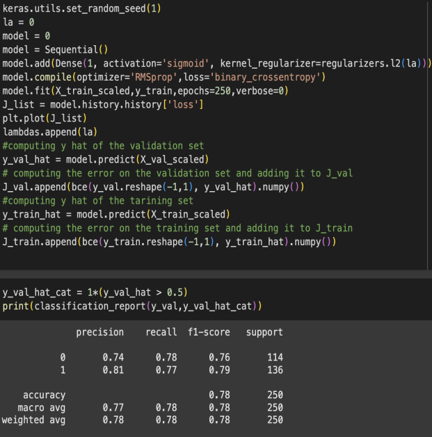
Figure 1: Results

Figure 1 shows results. After selecting the method and loss function, he model is constructed as illustrated. Initially, this model implemented a single layer, treating it as a regression problem with a sigmoid activation function. The number of epochs represents the steps through the training dataset; excessive epochs can cause overfitting, while insufficient epochs may result in underfitting. Next, I evaluated the model's accuracy on the validation set, which is the dataset aim to interpret. The accuracy reached 78%, indicating a decent performance, but there is potential for improvement by increasing the number of steps or layers. Consequently, Adding hidden layer to the model, maintaining the sigmoid activation function.

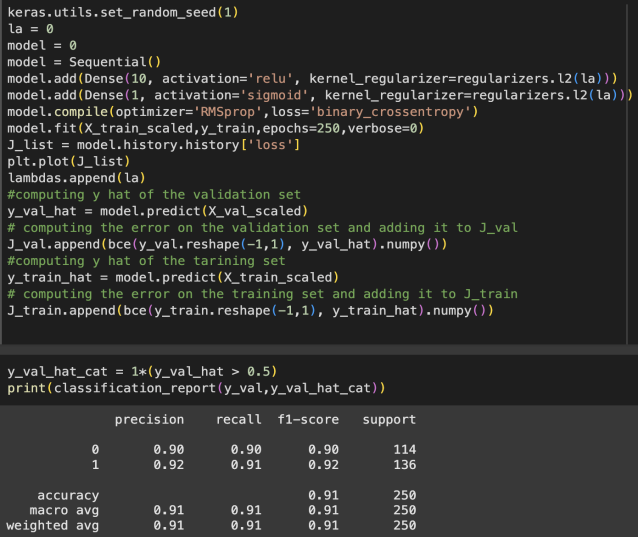
Figure 2: Results

Figure 2 shows that after running the new model, the result of accuracy is 91%

The 91% accuracy of this model is impressive. From 78% to 91%, The model only has one layer. This is a good example that combined all the concepts discussed before and improved the model's accuracy.

5. Conclusion

This paper analyzed three supervised learning algorithms—linear regression, decision trees, and neural networks—alongside the loss function. It showcased a neural network's application to emphasize the importance of supervised learning concepts and improving model prediction accuracy. The results reveal that each algorithm has unique strengths and weaknesses based on data characteristics and context: linear regression is ideal for linear problems, decision trees cater to both classification and regression, and neural networks offer flexibility and robustness for nonlinear, high-dimensional data. The main contribution of this paper is the introduction of supervised learning and its applications, including college prediction. It highlighted the effects of feature engineering, model selection, and optimization on model accuracy. Limitations included a scarcity of resources on supervised learning introductions. Nonetheless, supervised learning is poised to be a focal point in human development. Future research will aim to enhance model efficiency, particularly with large datasets and unbalanced classes. Additionally, integrating domain-specific knowledge into machine learning models can boost predictive performance in areas like medical diagnosis, materials science, and box office prediction. [10]

References

[1]. Nasteski, V. (2017). An overview of the supervised machine learning methods. Horizons. b, 4(51-62), 56.
[2]. Liu Duanyang, & Wei Zhongming. (2023). Application of supervised learning algorithms in materials science. Frontiers of Data and Computing, 5(4), 38-47.
[3]. James, G., Witten, D., Hastie, T., & Tibshirani, R. (2013). An introduction to statistical learning (Vol. 112, p. 18). New York: Springer.
[4]. Hao Zhihui. (2019). Comparative empirical analysis of stock price prediction based on supervised learning and unsupervised learning (Master's thesis, Shandong University). Master's degree
[5]. Hastie, T., Tibshirani, R., Friedman, J., Hastie, T., Tibshirani, R., & Friedman, J. (2009). Overview of supervised learning. The elements of statistical learning: Data mining, inference, and prediction, 9-41.
[6]. Hennig, C., & Kutlukaya, M. (2007). Some thoughts about the design of loss functions. REVSTAT-Statistical Journal, 5(1), 19-39.
[7]. Chai, T., & Draxler, R. R. (2014). Root mean square error (RMSE) or mean absolute error (MAE). Geoscientific model development discussions, 7(1), 1525-1534.
[8]. Mao, A., Mohri, M., & Zhong, Y. (2023, July). Cross-entropy loss functions: Theoretical analysis and applications. In International conference on Machine learning (pp. 23803-23828). PMLR.
[9]. Cunningham, P., Cord, M., & Delany, S. J. (2008). Supervised learning. In Machine learning techniques for multimedia: case studies on organization and retrieval (pp. 21-49). Berlin, Heidelberg: Springer Berlin Heidelberg.
[10]. Li Wangze. (2020). Research on the influencing factors of domestic film box office based on supervised learning (Master's thesis, Hubei University of Technology). Master's degree https://link.cnki.net/doi/10.27131/d.cnki.ghugc.2020.000459doi:10.27131/d.cnki.ghugc.2020.000459.
Cite this article
Jiao,H. (2025). Application of Supervised Learning Algorithms in Data Prediction. Applied and Computational Engineering,133,121-127.
Data availability
The datasets used and/or analyzed during the current study will be available from the authors upon reasonable request.
Disclaimer/Publisher's Note
The statements, opinions and data contained in all publications are solely those of the individual author(s) and contributor(s) and not of EWA Publishing and/or the editor(s). EWA Publishing and/or the editor(s) disclaim responsibility for any injury to people or property resulting from any ideas, methods, instructions or products referred to in the content.
About volume
Volume title: Proceedings of the 5th International Conference on Signal Processing and Machine Learning
© 2024 by the author(s). Licensee EWA Publishing, Oxford, UK. This article is an open access article distributed under the terms and
conditions of the Creative Commons Attribution (CC BY) license. Authors who
publish this series agree to the following terms:
1. Authors retain copyright and grant the series right of first publication with the work simultaneously licensed under a Creative Commons
Attribution License that allows others to share the work with an acknowledgment of the work's authorship and initial publication in this
series.
2. Authors are able to enter into separate, additional contractual arrangements for the non-exclusive distribution of the series's published
version of the work (e.g., post it to an institutional repository or publish it in a book), with an acknowledgment of its initial
publication in this series.
3. Authors are permitted and encouraged to post their work online (e.g., in institutional repositories or on their website) prior to and
during the submission process, as it can lead to productive exchanges, as well as earlier and greater citation of published work (See
Open access policy for details).