1. Introduction

Image filtering is an essential operation in image processing and computer vision. It refers to removing noise or undesired signals in the image without harming the general qualities of the original picture. According to the frequency distribution, the noise signal is composed of impulse noise, salt and pepper noise, and Gaussian noise. Among them, the characteristic of impulse noise is that the burst pulse amplitude is large, but the duration is short, and the interval between two impulse noises is long[1]. Bipolar impulse noise, also known as salt and pepper noise, is characterized by a random distribution of black and white on an image. The broadest noise is Gaussian noise in the form of Gaussian distribution. Therefore, numerous filtering methods are proposed to eliminate this noise for better image and video quality.

Typical image filtering methods consist of the median filter, mean filter, Gaussian filter, and K-nearest neighbor smoothing filter for different types of noise. The median filter is good at filtering impulse interference and salt and pepper noise, while the mean filter is typically used to deal with particle noise. The Gaussian filter has a better filtering effect on Gaussian noise. In addition, the K-nearest neighbor smoothing filter has the capability of boundary preservation. However, these traditional methods cannot obtain satisfied denoising results for different circumstances.

To further filter the noise, researchers present more effective algorithms. In [2], Wang et al. proposed a non-local means filter (NLM) combined with median filtering and an adaptive smoothing coefficient method. NLM can be used in mixed noise and further develop the denoising impact of the picture.

In [3], a more effective adaptive median filtering technique is suggested. Through two noise detections, the method identified the actual noise sites and the local noise density. The filter window size was then chosen in accordance with the density. Finally, the actual noise spots are filtered using the suggested procedure. According to the experimental findings, the enhanced adaptive median filter outperforms both the standard and adaptive median filters in terms of filtering performance.

Since the Gaussian filter cannot protect the edge of the image well, Tomasi and Manduchi [4] first designed the bilateral filter in 1998. The bilateral filter is non-linear and non-iterative. The innovation of the bilateral filter is that the impact of pixel value difference is considered based on a Gaussian filter, which drives the bilateral filter to perform well in smoothing images. The bilateral filter is an incredible and notable filter with an "edge-preserving & denoising" capability. Because of the qualities of the bilateral filter and its good complexity, it is utilized in numerous different fields, like image noise reduction, geological exploration, dehazing, sharpness enhancement, image editing, and medical magnetic resonance imaging. Thus, this paper focuses on the bilateral filter algorithm and its characteristic study for comprehensive analysis and better future applications.

Typical bilateral filtering optimization schemes can be separated into algorithm optimization and hardware optimization. For better results, bilateral filtering optimization algorithms usually consider the filtering window size optimization and filtering parameters optimization, while the latter plays a significant role. How to choose the appropriate parameters is the current focus of researchers.

According to the different methods of bilateral filtering, different filtering parameter optimization algorithms are proposed for image [5-10] and video applications [11-13], respectively. On the one hand, various methods are devoted to image filtering with spatial and frequency domain consideration. An adaptive parameter algorithm for bilateral filtering was proposed in [5]. This new algorithm could adaptively adjust the filtering parameters and achieve a good filtering effect. Experiments showed that this method could effectively remove image noise and detect actual edges. In [6], the authors proposed an algorithm to optimize bilateral filter parameters. The proposed algorithm utilized inputs such as noise density, edges, and histogram of the image to adjust the parameters. Experiments showed that the improved bilateral filter could effectively remove impulse noise. A general optimization algorithm was presented in [7] for better filtering outputs. The image containing Gaussian white noise was handled by adjusting the bilateral filter's two parameters. The algorithm also achieved positive outcomes on magnetic resonance imaging and multispectral and hyperspectral images. The Butterworth high-pass filter was combined with a bilateral filter to optimize bilateral filtering in the frequency domain in [8]. The suppression of interference improved the filtering performance of the bilateral filter and achieved a decent background suppression effect in the preprocessing of faint infrared marks.

Besides these methods, better bilateral filtering results are obtained in [9,10] by optimizing the Gaussian kernel into account for image filtering. In [9], researchers presented bilateral filtering with Elliptic Gaussian Kernel. Experiments showed that, compared with a standard bilateral filter, the proposed method could significantly reduce the amount of computation required while having high denoising quality and has made progress in seismic image processing. Chen et al. designed a novel Gaussian adaptive bilateral filter in [10], the basic idea of which was to obtain low-pass guidance of a range kernel through a Gaussian spatial kernel. According to experiments, it successfully speeded up the filter and adaptively got pure Gaussian range kernels for input images within different noise.

On the other hand, some novel parameter optimization methods were introduced for better video filtering [11-13]. The author proposed a parameter optimization algorithm in [11], which successfully accelerated bilateral filtering in the time domain and achieved better filtering results. For better handling of video images, an adaptive bilateral interpolation filter was proposed in [12], whose main innovation was to upsample the video or image by an arbitrary upsampling factor. The proposed algorithm was more effective in removing artifacts than the traditional upsampling method. In [13], an improved bilateral filter was applied to video coding, which could be utilized in temporal prediction of subsequent blocks and achieve better filtering effect.

It should be noted that the above algorithms are mainly aimed at software optimization. In practical applications, hardware bilateral filtering should meet real-time requirements. Therefore, further research on hardware structure design is required in addition to algorithm optimization.

Typical hardware optimizations include hardware fast algorithms optimizations and hardware structure optimizations. For better filtering results, fast hardware algorithms are based on various approximations of bilateral filters, such as fast algorithms [14]-[17]. For example, on the one hand, in [14] and [15], it is shown that researchers can reduce the complexity by quantifying the dynamic range of the original pictures. On the other hand, in [16] and [17], researchers demonstrate that fast bilateral filtering can be achieved by directly estimating the range kernel with trigonometric and polynomial functions.

Besides these above, the bilateral filtering hardware structure includes Field Programmable Gate Array(FPGA) and Very Large Scale Integration(VLSI) oriented designs. Several FPGA implementations of bilateral filters have been reported in [18]-[20] to improve the speed of bilateral filtering. FPGA implementations have been reported in [18] and [19]. The FPGA implementation in [20] was carefully optimized for memory and speed, while [19] employed a straightforward brute force approach. In [20], Vinh et al. tried to accelerate the implementation by substituting a piecewise polynomial for the Gaussian range kernel, which is less computationally expensive than going beyond Gaussian.

In addition, the authors proposed a low-cost VLSI architecture for bilateral filters in [21] for real-time image processing. The proposed architecture was cost-effective while preserving the same image quality, frame rate, and operational clock frequency, according to experimental findings.

This paper will concentrate on a top-to-bottom investigation of every strategy's qualities and progress drifts and propose conceivable future advancement bearings and trends to have a more efficient and exhaustive comprehension of the bilateral filter and its improvement. The remainder of this paper will be organized as follows. Section II will present the related research fields of bilateral filter optimization algorithms exhaustively, while the hardware design of bilateral filters will be investigated in Section III. Section IV will summarize and give the future prediction of the advancement heading of bilateral filtering.

2. Bilateral filter optimization algorithm

2.1. Bilateral filter review

Gaussian filtering will blur the edges of the image because only the position information is concerned in the filtering process. For example, in the window centered on \( q \) , the calculation method of the weight of a particular point \( p \) in the Gaussian filter is shown in (1),

\( G(p) = \frac{1}{2π{σ^{2}}}{e^{-\frac{{|p-q|^{2}}}{2{σ^{2}}}}} \) (1)

where the \( {σ^{2}} \) is the model parameter. In the filtering window, the weight of the point closer to the center point is more significant. However, in the edge area, since the difference in pixel values ​​on both sides of the edge is too large, Gaussian filtering will blur the edge information. Subsequently, to better protect the border, bilateral filtering was proposed.

Bilateral filtering is based on Gaussian filtering. The purpose is to protect the edge blurred by Gaussian filtering. It is a compromise process that combines the image’s spatial proximity and pixel values’ similarity. At the same time, spatial information and grayscale similarity are considered to achieve edge preservation.

A bilateral filter is a combination of spatial domain filtering and value domain filtering. Based on Gaussian filtering, pixel value weight \( {G_{r}} \) is proposed, and the spatial distance weight is expressed as \( {G_{s}} \) ,

\( {G_{r}} = {e^{-\frac{{|{I_{p}} - {I_{q}}|^{2}}}{2{{σ_{r}}^{2}}}}} \) (2)

\( {G_{s}} = {e^{-\frac{{|p - q|^{2}}}{2{{σ_{s}}^{2}}} }} \) (3)

where \( {σ_{s}} \) and \( {σ_{r}} \) denote the standard deviation over space and derivation in an edge's amplitude's intensity, respectively. The \( (p,q) \) is coordinate of each pixel and I is value of pixels .The filtering result \( BF \) is expressed as,

\( BF= \frac{1}{{W_{q}}}\sum _{p∈S}{G_{s}}(p){G_{r}}(p)* {I_{p}} \) (4)

\( = \frac{1}{{W_{q}}}\sum _{p∈S}{e^{-\frac{{|p - q|^{2}}}{2{{σ_{s}}^{2}}} }}*{ e^{-\frac{{|{I_{p}} - {I_{q}}|^{2}}}{2{{σ_{r}}^{2}}}}} * {I_{p}} \) (5)

where \( S \) is the neighborhood area and \( {W_{q}} \) is the weighted sum of each pixel value in the current filter window, which plays a normalizing role as,

\( {W_{q}}= \sum _{p∈S}{e^{-\frac{{|p - q|^{2}}}{2{{σ_{s}}^{2}}} }}*{e^{-\frac{{|{I_{p}} - {I_{q}}|^{2}}}{2{{σ_{r}}^{2}}}}} \) (6)

From the above formula, we can infer the following conclusion. In the flat region, since the difference between the pixel values of adjacent pixels is small, the spatial distance weight \( {G_{s}} \) plays a significant role, which is equivalent to directly applying Gaussian blur. And in the edge area, the \( {G_{r}} \) value on both sides of the edge distinguish a lot while inducing little effect on the filtering result. Therefore, bilateral filtering can effectively protect edge information.

2.2. Typical bilateral filtering optimization

According to the different optimization methods of bilateral filtering in images or videos, in this paper, we choose three typical approaches, which accelerate bilateral filtering in the frequency domain [8], spatial domain [10], time domain [13], respectively.

To improve the effect of image processing with no apparent shape and texture information, such as the air background’s weak and small infrared targets, in [8], the authors proposed a bilateral filter preprocessing algorithm combined with a Butterworth high-pass filter, which effectively improved the performance of the bilateral filter in the frequency domain.

In [8], the authors converted the original image to the frequency domain by Fourier transform to acquire \( F(x,y) \) where most of the background clutter was concentrated in the low-frequency domain. The target point was set as \( (x,y) \) and its neighborhood were \( (i,j) \) . Then the Butterworth high pass filter \( H(u,v) \) was utilized to handle the \( F(x,y) \) to eliminate the background clutter. The Butterworth high pass filter was as follows,

\( H(u,v)=\frac{1}{1+[\sqrt[]{2}-1]{[\frac{{D_{0}}}{D(u,v)}]^{4}}} \) (7)

where \( D(u,v) \) was the distance between the midpoint \( (u,v) \) in frequency domain space and the origin of frequency domain and \( {D_{0}} \) was the cutoff frequency.

After filtering, the majority of the target and noise were in the high-frequency range, and we could obtain image \( f(x,y) \) successfully by Fourier inverse Transform. Then \( f(x,y) \) is filtered by the enhanced bilateral filter (8) to obtain the image \( g(x,y) \) . The output of the enhanced bilateral filter can be computed as follows,

\( g(x,y)=\frac{1}{{W_{q}}}\sum _{i,j∈{N_{x,y}}}{e^{\frac{-[{(i-x)^{2}}+{(j-y)^{2}}]}{2{{σ_{d}}^{2}}}}}{e^{\frac{|F{(i,y)^{2}}+F{(x,y)^{2}}|}{2{{σ_{r}}^{2}}}}}×M×F(i,j) \) (8)

\( M=[ \begin{array}{c} \begin{matrix}1 & 1 & 1 \\ \end{matrix} \begin{matrix}1 & 1 \\ \end{matrix} \begin{matrix}1 & 1 \\ \end{matrix} \\ \begin{matrix}1 & 1 & 0 \\ \end{matrix} \begin{matrix}0 & 0 \\ \end{matrix} \begin{matrix}1 & 1 \\ \end{matrix} \\ \begin{matrix}1 & 0 & 0 \\ \end{matrix} \begin{matrix}0 & 0 \\ \end{matrix} \begin{matrix}0 & 1 \\ \end{matrix} \\ \begin{matrix}1 & 0 & 0 \\ \end{matrix} \begin{matrix}0 & 0 \\ \end{matrix} \begin{matrix}0 & 1 \\ \end{matrix} \\ \begin{matrix}1 & 0 & 0 \\ \end{matrix} \begin{matrix}0 & 0 \\ \end{matrix} \begin{matrix}0 & 1 \\ \end{matrix} \\ \begin{matrix}1 & 1 & 0 \\ \end{matrix} \begin{matrix}0 & 0 \\ \end{matrix} \begin{matrix}1 & 1 \\ \end{matrix} \\ \begin{matrix}1 & 1 & 1 \\ \end{matrix} \begin{matrix}1 & 1 \\ \end{matrix} \begin{matrix}1 & 1 \\ \end{matrix} \end{array} ] \) (9)

where \( {N_{x,y}} \) was the neighborhood area of (x, y)， \( M \) was the added filter template, represented by a matrix(9). Finally, \( f(x,y) \) and \( g(x,y) \) were differentiated to suppress background clutter.

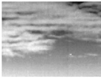
Figure 1. Original image [8].

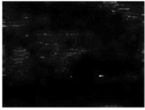
Figure 2. Processing result image [8].

The comparison results were shown in Figure 1 and Figure 2, which were this algorithm's original image and processing results. As could be seen, the proposed image preprocessing technique produced remarkable results. The majority of the cloud backdrop might be removed using the picture preparation approach suggested in this paper.

Secondly, the authors proposed a novel Gaussian adaptive bilateral filter(GABF) in [10] to optimize the filtering performance. The process was as follows. Firstly, as to the spatial domain method, a low-pass guidance picture by Gaussian blur process was generated as,

\( f(p)=\sum _{q}M_{p,q}^{g}(g){I_{q}} \) (10)

where \( {M_{p,q}} \) denoted the filter kernels at positions \( p \) and \( q \) of the guide image and \( g \) , and \( I \) represented guidance and input images, respectively. For the original image \( I \) , a Gaussian blur process, which corresponded to low-pass filtering, was utilized to produce a low-pass picture \( f(p) \) .

The primary distinction between GABF and conventional bilateral filters was that \( g \) and \( I \) were unique. The authors made sure that the inputs for the noise filtering weren't similar for \( g \) and \( I \) . And the Gaussian range kernel defined the impact of pixels from low-pass guiding \( {\bar{g}_{q}} \) which were derived from the Gaussian blur process on \( {I_{p}} \) , while the Gaussian spatial kernel was utilized on filtering input \( I \) .

Hence, the kernel of GABF was defined as,

\( M_{p,q}^{gabf}(I,\bar{g})=\frac{1}{{W_{q}}}exp⁡(-\frac{{||p-q||^{2}}}{{{σ_{s}}^{2}}})exp⁡(-\frac{{||{I_{p}}-{\bar{g}_{q}}||^{2}}}{{{σ_{r}}^{2}}}) \) (11)

Where the low-pass guidance \( \bar{g} \) came from (10). Although the filtering input \( I \) was tainted by various noise compositions, the Gaussian spatial kernel on \( I \) and Gaussian range kernel from \( \bar{g} \) enforced a rigorous preservation of image edges and contours while smoothing surfaces of objects in the filtering output \( f(p) \) . Consequently, the definition of the GABF output \( f(q) \) was,

\( f(p)=\sum _{q}M_{p,q}^{gabf}(I,\bar{g}){I_{q}} \) (12)

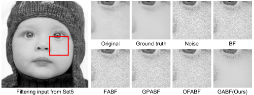
Figure 3. Input and output pictures from different filters [10].

Figure 3. showed that after the Bilateral Filter(BF), Fourier Approximation based BF(FABF), Gaussian Polynomial Approximation based BF(GPABF), and Optimized Fourier Approximation based BF(OFABF) were applied to it. Many noise artifacts remained in the image, and these methods clearly failed to recover a clean low-pass image. It was clear that GABF yielded the best results. The experimental results showed that GABF had a better smoothing function than ordinary bilateral filtering in the face of noise disturbance input.

Thirdly, an improved bilateral filter was proposed in [13] as a tool for video coding in the temporal domain to eliminate ringing artifacts in videos. The proposed method added inverse transform residuals to prediction and then directly applied to filter to achieve temporal prediction of subsequent blocks. The principle of this filter was as follows.

In order to reduce the impact on the signal while filtering out the ringing noise. The authors rewrote (5) as,

\( {I_{F}}=\frac{{ω_{C}}{I_{C}}+{ω_{A}}{I_{A}}+{ω_{B}}{I_{B}}+{ω_{L}}{I_{L}}+{ω_{R}}{I_{R}}}{{ω_{C}}+{ω_{A}}+{ω_{B}}+{ω_{L}}+{ω_{R}}} \) (13)

where \( {ω_{C}} \) was the weight for the center sample and \( {ω_{A}} \) , \( {ω_{B}} \) , \( {ω_{L}} \) , and \( {ω_{R}} \) , respectively, were the weights for the samples above, below, left, and right. The sample values for the samples above ( \( {I_{A}} \) ), below ( \( {I_{B}} \) ), left ( \( {I_{L}} \) ), and right ( \( {I_{R}} \) ) were combined to form the output sample value \( {I_{F}} \) . Their weights were set to zero for samples that weren't inside the transform block. The center weight \( {ω_{C}} \) was equal to 1. The other weights could be calculated by,

\( ω={e^{- \frac{1}{2{{σ_{s}}^{2}}}- \frac{{|∆I|^{2}}}{2{{σ_{r}}^{2}}}}} \) (14)

where \( ∆I \) was the intensity difference from the center sample. In [13] \( {σ_{s}} \) was defined as,

\( {σ_{s}}=μ-\frac{min{(width,height,16)}}{40} \) (15)

where \( μ \) = 0.92 for intra predicted blocks and \( μ \) = 0.72 for inter predicted block with \( width \) and \( height \) as the block width and height, respectively. To avoid excessive filtering, the authors chose a weaker filter and set \( {σ_{r}} \) based on the quantization parameter (QP) utilized in the current block as,

\( {σ_{r}}=max⁡(\frac{QP-17}{2},0.01) \) (16)

Every transform block was immediately filtered once the projected values for the block in the encoder and decoder were combined with the reconstructed residual values. As shown in Figure 4, the dark brown ringing pixels above the yellow area were suppressed.

The above three typical bilateral filtering optimization methods improved the quality of filtering images or videos from the frequency, spatial and temporal domains, respectively. It can be seen that all of them employ effective methods to achieve various adaptive parameters optimization for bilateral filtering, which obtains remarkable filtering performance. However, these methods are too complex for real-time processing, especially for hardware design. Therefore, hardware-friendly fast bilateral filtering algorithms and architecture should be further researched.

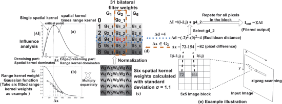
Figure 5. Algorithm framework of the piecewise approximation method [22].

3. Bilateral filter hardware friendly algorithm and architecture design

3.1. Overview of bilateral filtering gardware

Hardware implementation of bilateral filtering is crucial for real-time applications. Due to the nonlinear characteristics of bilateral filtering, the computational complexity of bilateral filtering is vast, and its hardware resources and computing complexity are proportional to its window size. So far, researchers have proposed several fast algorithms and hardware architectures to address the above problems. Real-time processing of large-scale, high-resolution photographs under strict hardware resource limitations is still a challenging task, nevertheless. This paper will focus on several typical fast algorithms and hardware structures of the bilateral filter.

3.2. Hardware friendly fast algorithms

To better incorporate the fast algorithm onto the hardware structure, in this paper, we study a typical hardware-friendly fast algorithm, which is a piecewise approximate computing algorithm [22].

To start with, a 5 × 5 filter mask was introduced in [22] as an example to describe the fast algorithm structure. The algorithm process was shown in Fig. 5. First, the authors analyzed the value difference on the output pixel in (5). This step demonstrated that a single spatial kernel made the output pixel( \( ∆I \) ) and the intensity difference( \( ∆x \) ) proportional. Still, a critical point would be generated after the spatial kernel was multiplied by the range kernel. It is now basically equivalent to that of a single spatial kernel. Next, the \( {G_{r}} \) in (2) was fitted according to the least squares method, and the analysis of the difference in the first step to protect the edge correctly. Before the critical point, the number of fitting points decreased because of the dominant spatial kernel, which was vital to reducing the storage of the look-up table (LUTs). The key point for piecewise approximation was determined to be at the average value. After the critical point, the output was dominated by the range kernel, increasing the proportion of fitting points. After that, the spatial weight's fitting point was multiplied by six range weights. Finally, the weight of the bilateral filter was created by normalizing the weights' product. The normalization process was as follows,

\( W_{q}^{ \prime }={W_{q}}×\frac{{W_{max}}}{\sum _{k,l}w(p,q,k,l)} \) (17)

where the normalized weight was \( W_{q}^{ \prime } \) and the sum of all the original weights was \( \sum _{k,l}w(p,q,k,l) \) . The \( (k,l) \) was the neighborhood coordinates of \( (p,q) \) and \( {W_{max}} \) was the upper limit of \( \sum _{k,l}w(p,q,k,l) \) .

The proposed piecewise approximation method precomputes the Gaussian function and approximates several fitting points as weights. The pre-calculated weights that are saved in LUTs ensure the filter processing acceleration. Therefore, it achieves optimization of computational cost and memory saving.

A typical hardware-friendly fast algorithm is described above which speeds up bilateral filtering to some extent. However, an excellent fast algorithm is required in practical applications, and the hardware structure adapted to it is equally important. Therefore, this paper will introduce two efficient bilateral filtering hardware structures.

3.3. Hardware structures

In addition to optimizing the fast algorithm for the hardware of bilateral filter, the researchers also optimized the hardware structures of bilateral filtering. This paper mainly lists two typical hardware structures: the FPGA architecture [23] based on a fast algorithm [17] and the VLSI architecture [21].

In [23], the authors proposed an FPGA architecture based on the fast algorithms presented in [17]. The representation of the overall architecture of the proposed FPGA structure was shown in Figure 6, where \( f(i) \) and \( {\hat{f}_{BF}}(i) \) represented the input and output images, respectively.

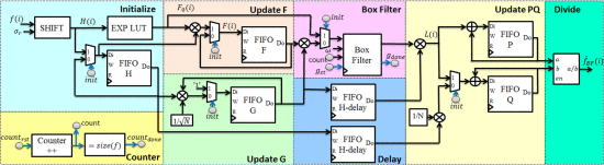
Figure 6. Overall FPGA architecture for the presented bilateral filter [23].

The lines highlighted in black with arrows represented the flow of picture data, while the lines in blue served as controls. The architecture's crucial scheduling component was in charge of timing the data flow between various blocks. The functional blocks in FPGA architecture were as follows: Initialize, Update F, Update G, Update PQ, Box Filter, Delay, and Counter, which were introduced in the fast algorithm[17]. Additional dormancy was introduced into the processing by the “Container” block, and the “Delay” blocks were utilized to make up for the inactivity. The “Counter” block synchronized the data flow between blocks.

The pictures were deposited in First In First Out(FIFO) blocks embedded in the Block Ram(BRAMs). They implemented read and write operations on the FIFO blocks to regulate the FIFO delays while controlling the data depth. Five FIFOs were utilized in the suggested architecture: "FIFO-H," "FIFO-F," "FIFO-G," "FIFO-P," and "FIFO-Q."

For a 256 \( × \) 256 size image, the proposed FPGA design required 2647 LUTS, 686 flip-flops(FF), 157 BRAM and 10 digital signal processing(DSP), while the maximum clock frequency was 60Mhz and the actual computation time was 18.93ms. The resource utilization and maximum clock frequency of the presented design were constant for different weights.

Besides the FPGA architecture, a VLSI architecture for bilateral filters was proposed. In [21], a VLSI hardware architecture of bilateral filters for current picture filtering was presented. This new low-cost VLSI architecture was described below.

The overall structure of this proposed VLSI hardware architecture is displayed in Figure 7. The original information in a filter window of size 5 \( × \) 5 was divided into six rows based on their distances from the central point. As shown in Figure 8, pixels with the same distance from the center point were set to one group.

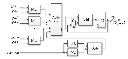
Figure 10. Circuit of kernel result calculation [21].

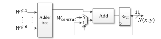
Figure 11. Circuit of normalization term calculation [21].

The authors' combined photometric and geometric weight calculation circuit is shown in Figure 9. The hardware architecture for the calculation of the normalization term and the kernel result was proposed in Figures 10 and 11, respectively. Finally, the normalization block calculated the output of the bilateral filtering was finished. \( g \) in Figs. 9–11 indicated the corresponding data group. The proposed design is implemented to achieve real-time bilateral filtering applications.

The proposed VLSI architecture required 5142 LUTS, 1782 look-up table-flip-flops (LUT-FF) pairs, 36 DSP, and 69 bonded Input Output Block(IOBS), while the maximum clock frequency was 236.697Mhz and the maximum frame rate was 56.43fps.

4. Conclusion

This paper analyzes several bilateral filtering optimization algorithms and hardware structures in detail, comparing their optimization methods and experimental results. The analysis results demonstrate that, according to the specific application scenarios, flexible adjustment of bilateral filtering parameters can effectively improve the performance of bilateral filtering. And hardware optimization can reduce hardware costs by designing an efficient hardware-friendly bilateral filtering algorithm or hardware structures. In the future, we can consider optimizing bilateral filtering parameters from the perspective of the human visual system and study the fast algorithm and hardware structures for the adaptive allocation of hardware resources based on corresponding application requirements.

References

[1]. H. M. Lin and A. N. W. Jr, “Median filters with adaptive length,” IEEE Transactions on Circuits and Systems, vol. 35, no. 6, pp. 675-690, June 1988.
[2]. S. Zhang and L. Wang, "An improved non-local means filter for image mixed noise," 2021 China Automation Congress (CAC), 2021, pp. 5545-5548.
[3]. J. Tang, Y. Wang, W. Cao and J. Yang, "Improved Adaptive Median Filtering for Structured Light Image Denoising," 2019 7th International Conference on Information, Communication and Networks (ICICN), 2019, pp. 146-149.
[4]. C. Tomasi and R. Manduchi, ‘‘Bilateral filtering for gray and color images,’’ in Proc. 6th Int. Conf. Comput. Vis., Jan. 1998, pp. 839–846.
[5]. C. Xiong, L. Chen and Y. Pang, "An Adaptive Bilateral Filtering Algorithm and its Application in Edge Detection," 2010 International Conference on Measuring Technology and Mechatronics Automation, 2010, pp. 440-443.
[6]. S. V. Priya and R. Seshasayanan, "Optimization of bilateral filter parameters for edge preserving impulse noise removal," 2015 International Conference on Computing and Communications Technologies (ICCCT), 2015, pp. 237-240.
[7]. I. Draganov and V. Gancheva, "Optimal Bilateral Filtering of CT Images," 2021 International Conference on Computational Science and Computational Intelligence (CSCI), 2021, pp. 1668-1672,
[8]. Z. Hu and Y. Su, "An infrared dim and small target image preprocessing algorithm based on improved bilateral filtering," 2021 International Conference on Computer, Blockchain and Financial Development (CBFD), 2021, pp. 74-77.
[9]. H. Nuha, M. Deriche and M. Mohandes, "Bilateral Filters with Elliptical Gaussian Kernels for Seismic Surveys Denoising," 2019 5th International Conference on Frontiers of Signal Processing (ICFSP), 2019, pp. 141-144.
[10]. B. -H. Chen, Y. -S. Tseng and J. -L. Yin, "Gaussian-Adaptive Bilateral Filter," in IEEE Signal Processing Letters, vol. 27, pp. 1670-1674, 2020,
[11]. Zengrong Lei and Zhuo Su, "Fast bilateral filtering using motion detection," 2011 International Conference on Image Analysis and Signal Processing, 2011, pp. 297-301.
[12]. Vanam, R., & Ye, Y. (2012). Adaptive bilateral filter for video and image upsampling. Applications of Digital Image Processing XXXV.
[13]. P. Wennersten, J. Strom, Y. Wang, K. Andersson, R. Sjoberg and J. Enhorn, "Bilateral filtering for video coding," 2017 IEEE Visual Communications and Image Processing (VCIP), 2017, pp. 1-4.
[14]. F. Durand and J. Dorsey, “Fast bilateral filtering for the display of highdynamic-range images,” ACM Trans. Graph., vol. 21, no. 3, pp. 257–266, 2002.A
[15]. Q. Y ang, K. H. Tan, and N. Ahuja, “Real-time O(1) bilateral filtering,” in Proc. IEEE Conf. Comput. Vis. Pattern Recognit., 2009, pp. 557–564.
[16]. K. N. Chaudhury, D. Sage, and M. Unser, “Fast O(1) bilateral filtering using trigonometric range kernels,” IEEE Trans. Image Process., vol. 20, no. 12, pp. 3376–3382, Dec. 2011.
[17]. K. N. Chaudhury and S. D. Dabhade, “Fast and provably accurate bilateral filtering,” IEEE Trans. Image Process., vol. 25, no. 6, pp. 2519–2528, Jun. 2016.
[18]. A. Gabiger-Rose, M. Kube, R. Weigel, and R. Rose, “An FPGA-based fully synchronized design of a bilateral filter for real-time image denoising,” IEEE Trans. Ind. Electron., vol. 61, no. 8, pp. 4093–4104, Aug. 2014.
[19]. H. Dutta, F. Hannig, J. Teich, B. Heigl, and H. Hornegger, “A design methodology for hardware acceleration of adaptive filter algorithms in image processing,” in Proc. IEEE Int. Conf. Appl.-Specific Syst., Arch. Processors, 2006, pp. 331–340.
[20]. T. Q. Vinh, J. H. Park, Y .-C. Kim, and S. H. Hong, “FPGA implementation of real-time edge-preserving filter for video noise reduction,” in Proc. IEEE Int. Conf. Comput. Electr . Eng., 2008, pp. 611–614.
[21]. C. -Y. Lien, C. -H. Tang, P. -Y. Chen, Y. -T. Kuo and Y. -L. Deng, "A Low-Cost VLSI Architecture of the Bilateral Filter for Real-Time Image Denoising," in IEEE Access, vol. 8, pp. 64278-64283, 2020,
[22]. R. Yao, L. Chen, P. Dong, Z. Chen and F. An, "A Compact Hardware Architecture for Bilateral Filter With the Combination of Approximate Computing and Look-Up Table," in IEEE Transactions on Circuits and Systems II: Express Briefs, vol. 69, no. 7, pp. 3324-3328, July 2022,
[23]. S. D. Dabhade, G. N. Rathna and K. N. Chaudhury, "A Reconfigurable and Scalable FPGA Architecture for Bilateral Filtering," in IEEE Transactions on Industrial Electronics, vol. 65, no. 2, pp. 1459-1469, Feb. 2018,
Cite this article
Lin,W. (2023). A survey of algorithm and hardware architecture for bilateral filter and application. Applied and Computational Engineering,4,768-779.
Data availability
The datasets used and/or analyzed during the current study will be available from the authors upon reasonable request.
Disclaimer/Publisher's Note
The statements, opinions and data contained in all publications are solely those of the individual author(s) and contributor(s) and not of EWA Publishing and/or the editor(s). EWA Publishing and/or the editor(s) disclaim responsibility for any injury to people or property resulting from any ideas, methods, instructions or products referred to in the content.
About volume
Volume title: Proceedings of the 3rd International Conference on Signal Processing and Machine Learning
© 2024 by the author(s). Licensee EWA Publishing, Oxford, UK. This article is an open access article distributed under the terms and
conditions of the Creative Commons Attribution (CC BY) license. Authors who
publish this series agree to the following terms:
1. Authors retain copyright and grant the series right of first publication with the work simultaneously licensed under a Creative Commons
Attribution License that allows others to share the work with an acknowledgment of the work's authorship and initial publication in this
series.
2. Authors are able to enter into separate, additional contractual arrangements for the non-exclusive distribution of the series's published
version of the work (e.g., post it to an institutional repository or publish it in a book), with an acknowledgment of its initial
publication in this series.
3. Authors are permitted and encouraged to post their work online (e.g., in institutional repositories or on their website) prior to and
during the submission process, as it can lead to productive exchanges, as well as earlier and greater citation of published work (See
Open access policy for details).