1. Introduction

With camera technology and computer science developing rapidly, demand for color images is increasing, and digital image processing is therefore becoming more and more important, especially color processing. Since almost any color can be obtained from the combination of red, green, and blue primary colors, this paper can store color images by recording the red, green, and blue information of each pixel in a matrix.

However, modern cameras usually obtain image information through CMOS (complementary metal oxide semiconductors) or CCDs (charge-coupled devices), which can only capture the light intensity of each pixel, but cannot know the light intensity of each pixel channel, so they can only create cameras that can take black-and-white photos or grayscale images. To record the red, green and blue information of each pixel, we need to add a color filter in front of the CCD, the most direct approach is to add different color filters, thus filtering out the colors of the three channels of RGB. However, with this method, it is necessary to apply three filters to each pixel to obtain the light intensity of three channels, and the cost is too high.

Modern engineering usually uses a Bayer filter [1] for CCDs to obtain red, green and blue color information. Instead of placing three color filters on each pixel, Kodak engineer Bryce Bayer, the inventor of the Bayer array, placed a single-color filter on each pixel at intervals. This way, it is possible to obtain a picture with partial values of each channel vacant. The ignored color of each pixel must be recovered from the neighboring pixels, a process known as color interpolation.

Many interpolation algorithms had been proposed successively, such as the bilinear algorithm, the Cok algorithm and the Hibbard-Laroche algorithm. However, the traditional interpolation algorithms may cause some problems, such as boundary effect, zipper effect and Moiré stripe effect. Since color image processing technology is especially important in computer vision fields such as cameras, virtual reality projection, 3D face recognition, and cell phone photography, and color interpolation algorithms are an important part of image processing and color imaging technology, exploring more accurate, efficient, and advanced color interpolation algorithms becomes an important grasp to improve color imaging performance. The traditional interpolation algorithms often have many unsatisfactory aspects.

This paper introduces and analyses three traditional interpolation algorithms, which are considered to be classical, in Section 2 (Related Work) and then proposes an improved algorithm in Section 3 to solve the problems mentioned above. Section 4 compares the advantages and disadvantages of these algorithms through experiments on Matlab, and finally conclude in Section 5.

2. Related works

The three classical interpolation algorithms are introduced and analysed in this section.

2.1. Bilinear interpolation

The bilinear interpolation [2] algorithm is the simplest interpolation algorithm and the basis for more advanced algorithms. The idea of the algorithm is that since the missing values of each pixel are likely to have similarity with the values of its neighbouring pixels, for any missing value, we look at its neighbouring pixels and take their average value if they contain one, then assign the calculated average value to the missing pixel. The detailed processes of the algorithm are as follows:

To recover the components of B and R on the G channel, peoples are able to get the average of the two B and two R values from the horizontal and vertical neighbors respectively. The formula is as follows:

\( \begin{matrix}{R_{i-1,j}}=\frac{{R_{i-2,j}}+{R_{i,j}}}{2}π \\ {B_{i-1,j}}=\frac{{B_{i-1,j-1}}+{B_{i-1,j+1}}}{2} \\ \end{matrix} \)

In the above formula: \( {R_{i,j}} \) stands for the value of red component of the pixel located at column \( j \) , row \( i \) , and so on. The B component on the R channel is obtained from the average of its four adjacent B values on the diagonal, and the G component is obtained from the average of its four horizontally and vertically adjacent G values. The other components on the B channel are recovered the same as on the R channel. The correlation among the three colors channels is ignored in bilinear interpolation, and its effect is relatively poor.

\( \begin{matrix}{B_{i,j}}=\frac{{B_{i-1,j-1}}+{B_{i-1.j+1}}+{B_{i+1,j-1}}+{B_{i+1,j+1}}}{4} \\ {G_{i-1,j-1}}=\frac{{G_{i-1,j-1}}+{G_{i,j-1}}+{G_{i-1,j-2}}+{G_{i-1,j}}}{4} \\ \end{matrix} \)

2.2. Cok interpolation

Through the argument of the physical optics Angle, we know that in a small smooth neighborhood of the same object, the light intensity ratio of the three color channels will not change very much. The Cok algorithm use the condition that the proportions among \( {R_{ij}} \) , \( {G_{ij}} \) and \( {B_{ij}} \) ( \( {R_{i,j,}}{B_{i,j}}and{G_{i,j}} \) )represent the coordinates of the red component, the green component and the blue component respectively)are equal to perform the interpolation algorithm . The algorithm first uses bilinear interpolation to calculate all the \( G \) components of the image，which is to fill out the green first. Then, the adjacent components are used to calculate the components pixels which are waiting to be solved. Finally, the average value is calculated by using multiple adjacent points. This method is to exclude the light and shade of the picture, increase the degree of color recovery, and increase the accuracy of interpolation. taking one of the pixels as an example, the formula is as follows：

\( {R_{i,j}}={G_{i,j}}×\frac{\frac{{R_{i-1,j-1}}}{{G_{i-1,j-1}}}+ \frac{{R_{i-1,j+1}}}{{G_{i-1.j+1}}}+ \frac{{R_{i+1,j-1}}}{{G_{i+1,j-1}}}+ \frac{{R_{i+1,j+1}}}{{G_{i+1,j+1}}}}{4} \)

Cok interpolation not only has a small amount of computation, but also can recover image information well. However, it also has obvious problems. From Equation (2.5), we know that G cannot be zero, in other words, this algorithm has a high requirement for the G component. When a computer computes, dividing by a smaller quantity produces a larger quantity, this will magnify the error caused by noise infinitely, and it will not be able to restore the obvious boundary areas in the picture well, so some degree of distortion are still remain which can be seen by eyes.

2.3. Gradient edge interpolation

Edge information is an important factor affecting the visual effect. It not only conveys most of the information of the image, but also outlines the basic contour of the object. Many image processing techniques rely directly or indirectly on the performance of edge detection algorithms [4], and applying edge detection technology to image interpolation can achieve good results.

This algorithm is mainly based on the idea of gradient [5]. That is, the gradient is detected first when the green channel is restored, and the interpolation direction is determined according to the gradient size. The reason is that if the direction with larger gradient is chosen for interpolation, it will greatly increase the possibility of color interpolation distortion; and if the idea of gradient is introduced, it can effectively reduce the appearance of color interpolation distortion. The Hibbard-Laroche algorithm(Two judgment formulas) is introduced for the calculation of the gradient.

Hibbard method is expressed as follows:

\( \begin{matrix}α=|{G_{3,2}}-{G_{3,4}}| \\ β=|{G_{2,3}}-{G_{4,3}}| \\ \end{matrix} \)

Laroche method is expressed as follows:

\( \begin{matrix}α=|2×{R_{3,3}}-{R_{3,1}}-{R_{3,5}}| \\ β=|2×{R_{3,3}}-{R_{1,3}}-{R_{5,3}}| \\ \end{matrix} \)

If α < β, there is a small possibility of a boundary in the horizontal direction and the interpolation is carried out along the horizontal direction as follows.

\( {G_{3,3}}=\frac{{G_{3,2}}+{G_{3,4}}}{2} \)

Vice versa is expressed as follows:

\( {G_{3,3}}=\frac{{G_{2,3}}+{G_{4,3}}}{2} \)

Another idea is the idea of constant color difference. When recovering the red and blue channels, the red and blue information is calculated by using the constant color difference in the small neighborhood. The color difference is usually R for red, B for blue and G for green. color difference constancy considers that the color difference is constant within a small smooth area of the image.

\( \begin{matrix}{R_{i,j}}-{G_{i,j}}={R_{m,n}}-{G_{m,n}} \\ {B_{i,j}}-{G_{i,j}}={B_{m,n}}-{G_{m,n}} \\ \end{matrix} \)

Then, the following formula is obtained:

\( {R_{i-1,j}}={G_{i-1,j}}+\frac{{R_{i-2,j}}-{G_{i-2,j}}+{R_{i,j}}-{G_{i,j}}}{2} \)

This class of algorithms can effectively reduce the processing imprecision brought by similar bilinear interpolation methods, but the results still fall short of expectations in some aspects such as edge processing. However, there are two obvious problems with the Hibbard-Laroche algorithm when probing edges using gradients. First, too little information is utilized to compute the gradient; the Hibbard method uses only the surrounding green pixel points, while the Laroche method uses only the surrounding red or blue pixel points. The gradient thus computed depends entirely on the information provided by the pixel points of a particular color and may differ significantly from the true gradient. In addition, interpolating to recover the green component simply assumes that the edges are oriented either along the horizontal or vertical direction, and directly interpolates either one of the horizontal or vertical directions, which is too idealistic.

3. Methodology

This paper optimize the Hibbard-Laroche algorithm and proposed a gradient edge interpolation algorithm considering weight based on the Sobel operator. There are some problems with the Hibbard-Laroche algorithm, which we try to solve in the improved algorithm. First, too little information is utilized to compute the gradient; the Hibbard method uses only the surrounding green pixel points, while the Laroche method uses only the surrounding red or blue pixel points. In addition, interpolating to recover the green component simply assumes that the edges are oriented either along the horizontal or vertical direction, and directly interpolates either one of the horizontal or vertical directions, which is too idealistic. The fact that the edge may have an arbitrary size angle with the horizontal line taken into consideration, it is more reasonable to interpolate the horizontal and vertical directions by assigning a certain weight to each of them, instead of choosing one of the two directions. For the problem that too little information is utilized in calculating the gradient, Sobel operator [6][7] is introduced to calculate the gradients to solve it. To solve the problem of interpolation edge direction selection [8][9], this paper calculate the interpolation weights of the two directions according to the relative magnitudes of the gradients in the horizontal and vertical directions.

3.1. Edge feature gradient calculation

The Sobel operator is a 3 × 3 convolution kernel that uses local differences to find edges and computes an approximation of the gradient. Sobel operators of x- and y-direction are given respectively below.

\( {G_{x}}=\begin{matrix}-1 & 0 & 1 \\ -2 & 0 & 2 \\ -1 & 0 & 1 \\ \end{matrix} \)

\( {G_{y}}=\begin{matrix}-1 & -2 & -1 \\ 0 & 0 & 0 \\ 1 & 2 & 1 \\ \end{matrix} \)

The gradient has a direction, and for an image, the approximation of the partial derivatives[10] in the horizontal and vertical directions can be computed by the Sobel operator respectively. Assume that the size of the original image is 3 × 3, as shown in Figure 1, then calculate the partial derivatives α in the horizontal direction at the point P5 as follows.

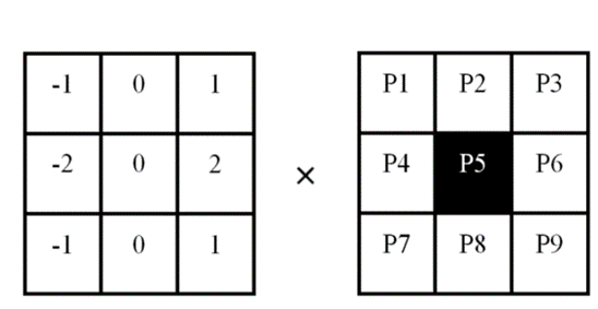
\( α=|({P_{3}}-{P_{1}})+2×({P_{6}}-{P_{4}})+({P_{9}}-{P_{7}})| \)

In a few words, the left pixels’ values of pixel point \( {P_{5}} \) are subtracted from the right pixels’ values and then the absolute value is taken, and the point near to \( {P_{5}} \) has a larger weight of 2; the point far from \( {P_{5}} \) has a smaller weight of 1. The partial derivative β in the vertical direction is calculated as follows.

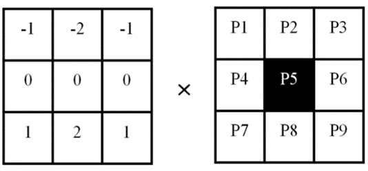
\( β=|({P_{7}}-{P_{1}})+2×({P_{8}}-{P_{2}})+({P_{9}}-{P_{3}})| \)

In a few words, the pixels’ values of the previous row of pixel point \( {P_{5}} \) are subtracted from the pixels’ values of the next row and then the absolute value is retained, and the weight of the point close to \( {P_{5}} \) is larger and is 2; the weight of the point far from \( {P_{5}} \) is smaller and is 1.

3.2. Gradient edge interpolation algorithm considering weight

The main algorithm flow chart in this section is as follows:

First of all, Through the operation in Section 3.2, the horizontal and vertical gradients of a given pixel. After the horizontal and vertical gradients are obtained by the Sobel operator, the interpolation weights of the two directions are converted according to the relative sizes of the horizontal and vertical gradients.

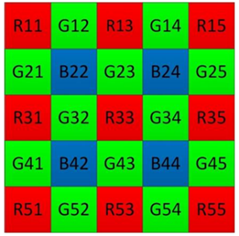
As show in Fig.4, taking the interpolation of the green component of R33 as an example, let its gradients in the horizontal and vertical directions be \( α \) and \( β \) , respectively, then this paper have:

\( {G_{33}}=\frac{α}{α+β}×\frac{{G_{23}}+{G_{43}}}{2}+\frac{β}{α+β}×\frac{{G_{32}}+{G_{34}}}{2}  \)

Here, \( {G_{33}} \) stands for the value of the green component of the pixel located at column 3, row 3, and so on. What’s more, \( α \) and \( β \) refer to the horizontal and vertical gradients of the given pixel respectively.

If the gradient in the horizontal direction is smaller, it means that the direction of the boundary is closer to the vertical direction, then the horizontal direction should account for a higher percentage in the interpolation, and vice versa. Obviously, the result given by equation Eq.14 meets such a requirement.

Note that before using Eq.14 for interpolation we should judge whether α + β is 0. If α + β = 0, since both are absolute values and thus are non-negative, which means that the gradient of both horizontal and vertical directions is 0. At this time, there is no edge near the pixel point, and 50% of each of the two directions can be interpolated, that is:

\( {G_{33}}=\frac{{G_{23}}+{G_{43}}+{G_{32}}+{G_{34}}}{4} \)

If α + β ≠ 0, interpolation is performed using Eq.14. The above operations are conducted on each pixel of the image to be processed so that the green information of all pixels can be recovered. After recovering the green component like this, the algorithm then recovers the red and blue components according to the same method of constant color difference as the Hibbard-Laroche algorithm, whereby the complete image information is obtained.

4. The evaluation of experiment

4.1. The method of quantitative index

The purpose of this experiment is to investigate the processing ability of the algorithm on Bayer color image, and use MATLAB to simulate. The interpolation effect of each algorithm is analyzed and compared from two indexes of visual effect and objective quality. In order to compare the image quality objectively，this paper use SSIM below, PSNR. and MSE as quantitative index，and they were tested for the Zipper effect. The calculation method of evaluation parameters is as follows:

\( SSIM=\frac{(2{μ_{f}}{μ_{\widetilde{f}}}+{C_{1}})(2{σ_{\widetilde{f}f}}+{C_{2}})}{(μ_{f}^{2}+μ_{\widetilde{f}}^{2}+{C_{1}})(σ_{f}^{2}+σ_{\widetilde{f}}^{2}+{C_{1}})} \)

In Eq.16, where \( {μ_{f}} \) and \( {μ_{\widetilde{f}}} \) represent the mean of the images \( f \) and \( \widetilde{f} \) , \( {σ_{f}} \) and \( {σ_{\widetilde{f}}} \) represent the variance of the images \( f \) and \( \widetilde{f} \) , respectively, and \( {σ_{f\widetilde{f}}} \) represent the covariance of the images \( f \) and \( \widetilde{f} \) .

\( PSNR=10{log_{10}}{\frac{MN}{{‖f-\widetilde{f}‖^{2}}}} \)

\( MSE=\frac{1}{MN}{\sum _{m=1}^{M}\sum _{n=1}^{N}‖f[m,n]-\widetilde{f}[m,n]‖^{2}} \)

In Eq.17 and Eq.18, \( M \) and \( N \) are the height and width of the image, respectively. Where \( M \) and \( N \) represent the size of the image as \( M \) rows and \( N \) columns, \( f[m,n] \) and \( \widetilde{f}[m,n] \) respectively represent the intensity components of the original image and the reconstructed image in row \( m \) and column \( n \) .

SSIM evaluates the similarity of two images from three aspects: brightness, structure and contrast. The degree of consistency between the interpolated image and the original image can be reflected by PSNR，and the degree of difference between the estimator and the estimator can be reflected by MSE. Both SSIM and PSNR indicate that larger values are better, while smaller MSE indicates better model quality and more accurate prediction.

4.2. The comparison of experimental results

In this experiment, many standard images are selected as the original sample images, and the four linear interpolation algorithms introduced in this paper are used to restore the color of the above color images. According to Eq.16, Eq.17 and Eq.18 to calculate the SSIM, PSNR, MSE which values of the restored image, and objectively compare the quality of the image. Partial experimental results are shown in Figures 5.

.

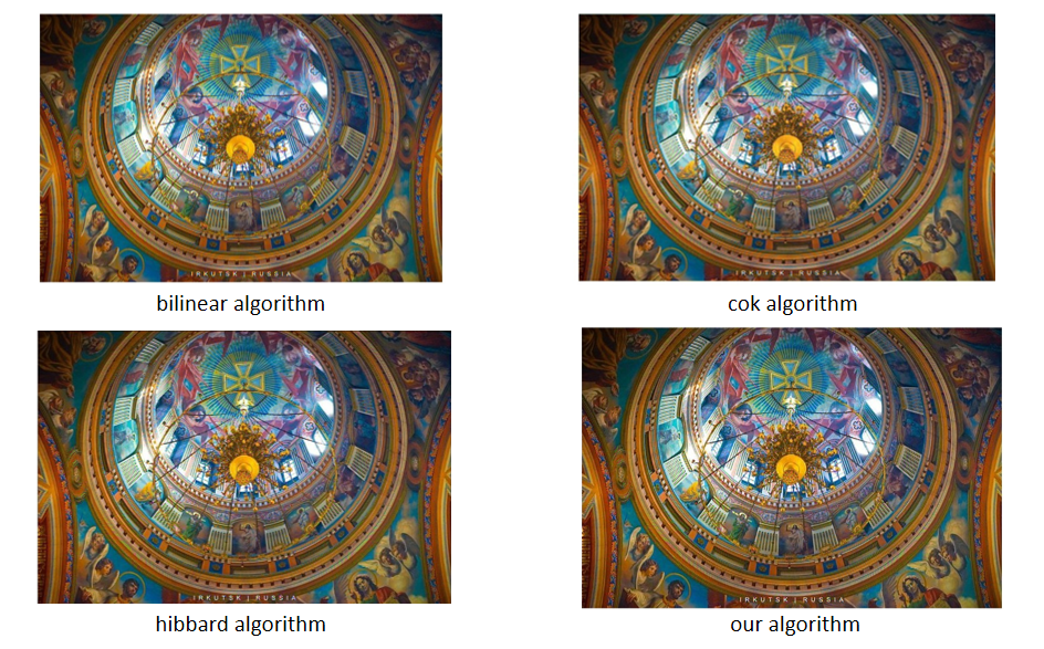
Figure 5. Simulation results of several difference algorithms.

Subsequently, this paper tested the zipper effect on another standard image, as shown in Fig.6.

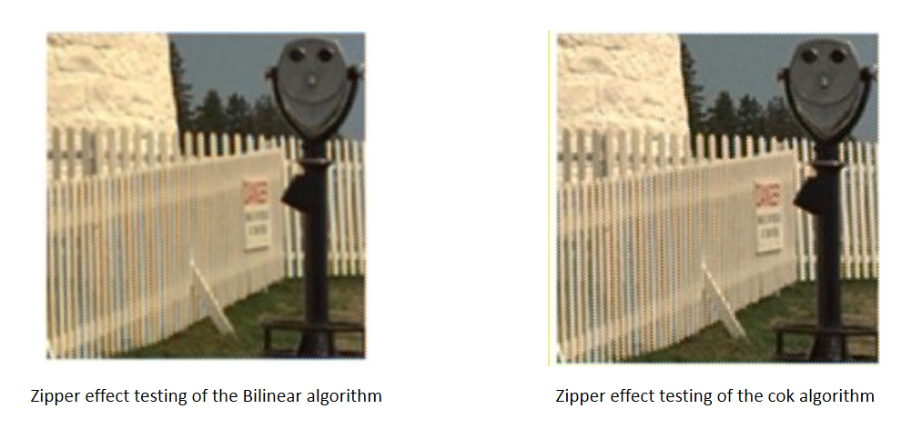
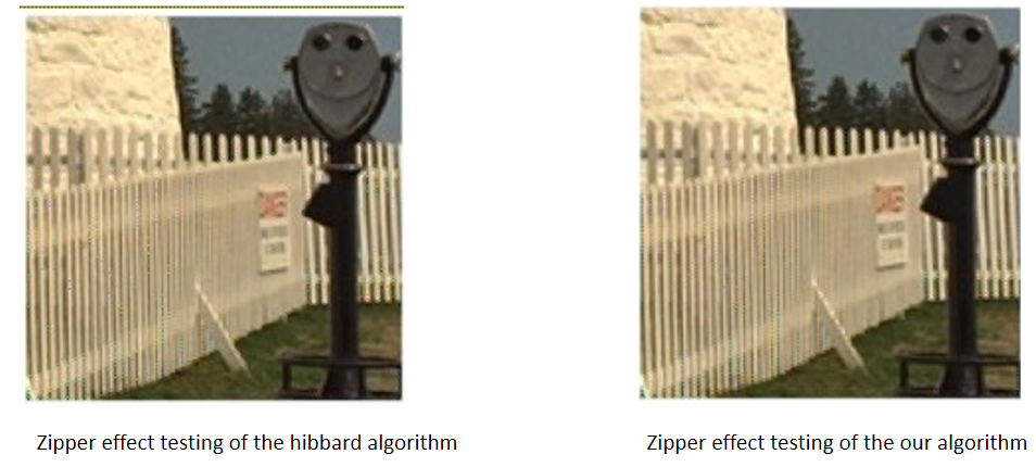
Figure 6. Zipper effect test of several algorithms.

Because the image is a complex scene image, it is difficult to visually distinguish the optimization effect. Therefore, this paper evaluates the experimental results through quantitative indicators in the next chapter.

4.3. The comparison of quantitative index

The comparative data of the experimental results in this paper are shown in Table 1.

Table 1. Quantization index of sample image.

By comparison, the SSIM and PSNR values of our improved algorithm are the highest, and the MSE is the smallest. As is shown in the Zipper effect test, our improved algorithm has the best restoration effect and the least noise. It can be seen that the role of convolution is not only to realize image blurring or denoising, but also to find all the gradient information on an image. Sobel operator has the advantages of strong anti-noise, no missing edge detection, no false edge detection and accurate positioning. Using weighted average algorithm and Sobel operator to calculate the gradient can effectively suppress the random noise of the image, and can provide more accurate edge direction information. This algorithm has a good effect on image processing with gray gradient and more noise, and effectively inherits the characteristics of bilinear interpolation for non-edge regions, which is faster and smoother.

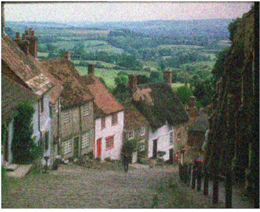
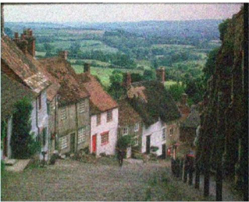
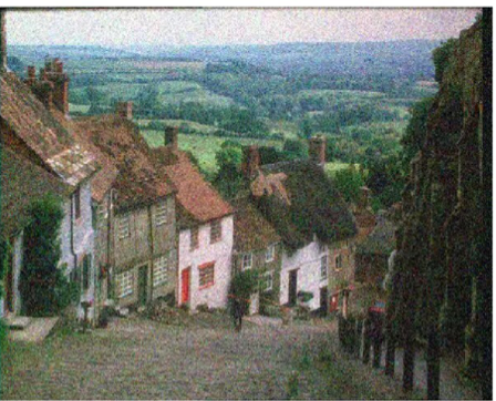
4.4. The processing ability of this algorithm for noisy images

In order to test the processing ability of the algorithm for noisy images, a rural scenery map (Fig.7.a) is processed with noise, and Gaussian noise[11] is added to obtain Fig.7.b Next, we use the Hibbard algorithm and our improved algorithm to restore Fig.7.b, obtaining Fig.7.c and Fig.7.d respectively. Then, Fig.7.c and Fig.7.d are respectively used as the reconstructed images, and the original image without noise (Fig.7.a) of the rural scenery is used as the original image to calculate the SSIM, PSNR and MSE, finally，the results are shown in Table 2.

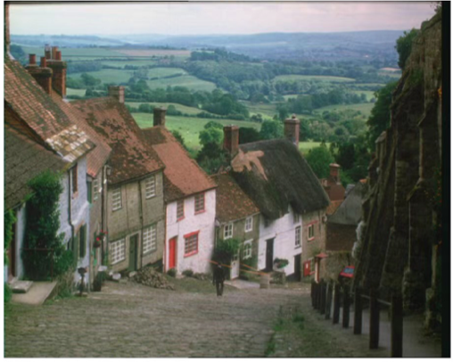
It can be seen that, compared with the results obtained by the gradient edge interpolation algorithm from the noisy image, the results obtained by our improved algorithm from the noisy image have higher similarity and smaller deviation with the original image without noise. This verifies that our algorithm has better anti-noise and de-noising ability.

Table 2 Experimental results of image denoising.

5. Conclusion

In this paper, an improved Hibbard interpolation algorithm, which using Sober operator to compute the gradients and assigns reasonable weights to both horizontal and vertical directions is proposed. As is verified by the experiments, our improved algorithm is obviously superior to the classical interpolation algorithms, in terms of subjective visual effect as well as objective evaluation indexes such as structural similarity index, peak signal-to-noise ratio and minimum mean square error. What’s more, our algorithm demonstrates better ability in procession of noisy images than the classical ones. It can be seen that our research generally lives up to the expectations and our novel interpolation algorithm can contribute to the development of demosaicing techniques, which really matters in the processing of images.

However, there’s still much room for our algorithm to progress. For instance, it makes no improvements on the second half of Hibbard interpolation, which recovers the red and blue information based on the idea of constant color difference. In addition, machine learning and deep learning can be introduced to restore specific patterns of images better in further improvement of interpolation algorithms. This paper believe that demosaicing techniques will keep progressing in the future.

References

[1]. S. Patil and P. Deepika (2019) Compression of Bayer Color Filter Array Images. In: 2019 4th International Conference on Recent Trends on Electronics, Information, Communication & Technology (RTEICT), 2019, pp. 281-284.
[2]. Li and Zhi qiang (2015) Bilinear and smooth hue transition interpolation-based bayer filter designs for digital cameras. In: International Journal of Circuits, Systems and Signal Processing, v 9, p 211-221, 2015; E-ISSN: 19984464.
[3]. Wang, Huan, Chen, Xianzhong and Hou Qingwen(2016)SAR imaging algorithm for the burden surface in BF based on cok algorithm. In: the World Congress on Intelligent Control and Automation (WCICA), Volume 2016-September, Pages 1436-1441.
[4]. Li Hui(2022) Multilevel Image Edge Detection Algorithm Based on Visual Perception In: Security and Communication Networks Volume 2022.
[5]. Yanhong Yang; Jianwei Zheng; Shengyong Chen (2020) Local low-rank matrix recovery for hyperspectral image denoising with ℓ 0 gradient constraint In: Pattern Recognition Letters Volume 135, 2020. PP 167-172.
[6]. Zhang, CC (Zhang, Chao-Chao); Fang, JD (Fang, Jian-Dong) (2016) Edge Detection Based on Improved Sobel Operator. In: ACSR-Advances in Computer Science Research Volume 52 Page 129-132.
[7]. Chung, Yunchu, Kim and Youngmin (2021) Comparison of Approximate Computing with Sobel Edge Detection. In: IEIE Transactions on Smart Processing and Computing, v 10, n 4, p 355-361, 2021; E-ISSN: 22875255.
[8]. Ge and Runchan (2022) A Design of Optimized Color Image Interpolation Algorithm Based on Edge Gradient. In: Proceedings - 2022 International Conference on Big Data, Information and Computer Network, BDICN 2022, p 708-712, 2022, Proceedings - 2022 International Conference on Big Data, Information and Computer Network, BDICN 2022 ISBN-13: 9781665484763.
[9]. Lu, Zhi-Fang; Zhong, Bao-Jiang (2018) Image Interpolation With Predicted Gradients. In: Zidonghua Xuebao/Acta Automatica Sinica, v 44, n 6, p 1072-1085, June 2018; Language: Chinese; ISSN: 02544156.
[10]. Hartmann Raphael; Klauer Karl Christoph(2021) Department of Psychology, University of Freiburg, D-79106 Freiburg, Germany; Department of Psychology, University of Freiburg Engel bergerstrasse, 41 Freiburg D-79106 Germany. In: Journal of Mathematical PsychologyVolume 103, 2021.
[11]. Baboshina, V.A., Orazaev, A.R, Shalugin, E.D. and Sinitca, A.M.(2022) Combined Use of a Bilateral and Median Filter to Suppress Gaussian Noise in Images. In: The 2022 11th Mediterranean Conference on Embedded Computing (MECO), pp. 5.
Cite this article
Chen,S.;Yin,S.;Zhao,Y. (2023). An improved hibbard interpolation algorithm based on edge gradient feature detection using Sobel operator. Applied and Computational Engineering,4,786-794.
Data availability
The datasets used and/or analyzed during the current study will be available from the authors upon reasonable request.
Disclaimer/Publisher's Note
The statements, opinions and data contained in all publications are solely those of the individual author(s) and contributor(s) and not of EWA Publishing and/or the editor(s). EWA Publishing and/or the editor(s) disclaim responsibility for any injury to people or property resulting from any ideas, methods, instructions or products referred to in the content.
About volume
Volume title: Proceedings of the 3rd International Conference on Signal Processing and Machine Learning
© 2024 by the author(s). Licensee EWA Publishing, Oxford, UK. This article is an open access article distributed under the terms and
conditions of the Creative Commons Attribution (CC BY) license. Authors who
publish this series agree to the following terms:
1. Authors retain copyright and grant the series right of first publication with the work simultaneously licensed under a Creative Commons
Attribution License that allows others to share the work with an acknowledgment of the work's authorship and initial publication in this
series.
2. Authors are able to enter into separate, additional contractual arrangements for the non-exclusive distribution of the series's published
version of the work (e.g., post it to an institutional repository or publish it in a book), with an acknowledgment of its initial
publication in this series.
3. Authors are permitted and encouraged to post their work online (e.g., in institutional repositories or on their website) prior to and
during the submission process, as it can lead to productive exchanges, as well as earlier and greater citation of published work (See
Open access policy for details).